1. Introduction

The urban heat island (UHI) effect, which is the presence of elevated temperatures in urban areas relative to their surroundings in the rural environment, has become one of the most characteristic anthropogenic climate change manifestations in recent times [1,2]. This phenomenon has grown more pronounced as the world urbanizes, with more than 68 $\%$ of the world's people projected to live in urban areas by 2050 [3] under the potential combined impact from ongoing climate change [4- 6]. In addition to impacting local climate patterns [7], the UHI effect also has profound implications for human health [8], energy consumption [9], and urban sustainability [10]. The UHI effect is a particularly pressing challenge in regions such as Greater Bay Area of China (GBAC) that are under rapid development [11]. As one of the world's fastest growing megacities and the core city of GBAC, the city of Shenzhen has expanded dramatically in the last four decades from small villages to a metropolitan area of more than 10 million people [12]. The city offers an ideal case study for investigating how urban climate is modified by such unprecedented fast urban development.

As UHI are one of the most important urbanization- induced modifications of the local climate [13], accurate mapping and analysis of these thermal variations at high resolutions are of great importance for urban climate research and planning [14]. Traditionally, many of the studies on UHI have relied on sparse networks of weather stations or low- resolution satellite observations and often miss the details of the fine scale spatial and temporal patterns of urban air temperature patterns. Nevertheless, recent progress in high resolution remote sensing technologies along with the creation of local climate zone (LCZ) classification systems [15] and machine learning techniques [16] have recently made the study of detailed urban thermal environment analysis possible [17,18]. These developments have offered opportunities to better quantify and understand UHI patterns in more precise terms and thus help inform urban planning and climate adaptation.

Despite significant progress in UHI research, current approaches still remain limited in terms of balancing spatial coverage and temporal resolution and often rely on extensive sensor networks that are

frequently impractical in many cities located at different latitudes, climate conditions, or socioeconomic development levels. At the same time, urban climate research still has a certain level of disconnection with practical applications such as urban building energy modeling [19], as current methods are missing the spatiotemporal resolution for detailed microclimate and energy analysis. Moreover, the predominant focus on mapping LST as a proxy for air temperature, rather than measuring air temperature itself, creates a significant gap between UHI research and its practical applications, since air temperature is the parameter that directly influences human thermal comfort [20] and building energy performance [21]. Here, a detailed literature review was conducted to show the status quo of current research progress in related fields in the following section.

2. Literature review

The evolution of UHI research has progressed significantly over recent decades, transitioning from basic insitu observations to advanced modeling approaches. Table 1 presents a chronological overview of key urban thermal environment related studies, highlighting their methodologies, spatial and temporal resolutions, etc. This overview provides context for the methodological advancements while clearly illustrating the research gaps our study aims to address. As shown in Table 1, UHI research has evolved different phases chronically, which we discuss in more detail below.

2.1. Early developments (2010-2015)

In the early 2010s, Zaksek and Ostir downscaled the LST data in urban area with the aim of analyzing the UHI diurnal cycle, showing that the SEVIRI data can be improved to deliver both high spatial and temporal resolutions [22]. Their method was particularly suited to capturing the dynamic nature of urban temperature variations over the course of the day, acting as a steppingstone for future research. At this time, spatiotemporal image fusion techniques were built upon this foundation, utilizing Landsat and MODIS images to produce high resolution temperature data [23]. The developed fusion approach was a major advance in the ability to continuously monitor UHIs with high spatial detail. Li and Bou- Zeid further advanced the field by developing the improved Princeton UCM and CZ09 parameterization using the WRF- PUCM model [24]. With the help of the enhanced model, surface temperature biases in UHI simulations were significantly reduced, and the creation of a more appropriate framework for understanding the dynamics of urban thermal processes.

2.2. Mid-decade advancements (2015-2018)

The mid 2010s witnessed the appearance of comprehensive long- term studies that revolutionized our knowledge of UHI dynamics. Shen et al. performed a 26 year analysis of Wuhan, China, finding that UHI intensity (UHII) does not follow simple trends of increase and decrease over long time scales [25]. For instance, their study was noteworthy to show that the relationships between heat distribution and land cover are interannual stable and that industrial activity is a dominant contributor to UHI effects. Providing crucial insight, Azevedo et al. compared satellite derived LST to high resolution air temperature observations in Birmingham, UK [26]. Their work showed that surface heat island distribution is fundamentally determined by land use patterns, and that reconciling multiple temperature measurement approaches can be challenging. Berger et al. analyzed the relationship between 2D/3D urban characteristics and the LST [27]. They found that while their relationships are temporally stable, which are subject to modulation by seasonal changes, phenology of vegetation and meteorological conditions. It was important work to the complex interplay between urban form and thermal patterns.

The related field also matured with review works and methodological improvements. Zhou et al. conducted a comprehensive systematic review of satellite remote sensing applications for surface UHIs and found that the Chinese studies are geographically concentrated as well as temporally focused on daytime summer conditions [28]. It is their work that helped identify methodological limitations and future research directions. Deilami et al.'s systematic review of spatio temporal factors expanded our understanding by detailed analysis of how vegetation cover, built up area, population density and water bodies impact UHI effects [29]. Their work is valuable at synthesizing all of the complex interactions between these various factors. Using WRF models, Li et al. [30] introduced an innovative method for the quantification of UHI using impervious surface area. Distinct diurnal patterns of their application to Berlin were shown with peak intensity at night. It provided insights in the temporal dynamics of UHIs and their relationship to surface characteristics.

2.3. Recent innovations (2019-Present)

In recent years, sophisticated technologies and machine learning approaches were integrated into UHI related research. Anjos et al. made important contributions by applying LCZ classification to the study of UHI behavior under different synoptic patterns [17]. By identifying six different LCZ sub classes, they also developed new frameworks to understand urban thermal patterns and their relationship to urban planning. Through their introduction of Tukey g- and- h random field models, Murakami et al. advanced the field and uncovered previously hidden heatwave structures in urban environments [31]. By innovatively incorporating higher order stochastic spatial properties, their work provided new tools for real time heatwave risk management. Chen et al. developed a high resolution monitoring approach based on random forest models and multi- platform observations [32]. This work was important in showing how wind patterns can determine the intensity of UHI, and for expanding our understanding of urban thermal dynamics. Zumwald et al. [33] employed crowd sensing data with machine learning for urban temperature mapping, and Zhang et al. [34] applied deep learning based methods to produce $500\mathrm{m}$ resolution spatiotemporally continuous air temperature data. Shi et al. [35] extended the field further with their Comprehensive Flexible Spatiotemporal Data Fusion Method (CFSDAF), which particularly excelled at retaining spatial information and restoring spatial continuity in the urban temperature measurement.

More recent research in this area has addressed remaining challenges and extending applications. Multiscale geographically weighted regression was employed by Luo et al. [36] to predict surface UHI and found that anthropogenic activity is the main driver of UHIs in Chengdu, China. The work also offered critical insights into the linkage between human activity and urban thermal regimes. In particular, Ding et al. have made contributions through their machine learning assisted mapping approach to address the issue of sparse meteorological data in urban climate modeling [37]. The work showed that machine learning techniques could generate high resolution temperature maps even with limited data inputs, which could be used to develop urban climate adaptation strategies. Zhang et al. contributed to the field by evaluating the all- weather LST reconstructed for UHI analysis in the Lhasa region [38]. They showed that all weather LST reconstruction was effective in capturing spatial distribution characteristics of UHIs, improving their accuracy for heat island effect governance. Hurduc et al. conducted comprehensive comparison of various satellite LST products, which not only showed substantial differences in their ability to capture surface UHI effects, but also gave important guidance to choose between different data sources for different types of UHI studies [39].

2.4. Research gaps and opportunities

As shown in Table 1, the evolution of UHI research in recent period is clear - that is from simple remote sensing applications to more complex

Table 1 Urban thermal environment studies: a chronological overview.

multiple source data integration and machine learning. Success has been achieved in moving the field toward ever higher spatial and temporal resolutions, with simultaneous understanding of the increasingly complicated interactions between urban form, human activity, and thermal patterns. New possibilities of urban temperature analysis are thus opened by the integration of traditional measurement methods with modern techniques such as crowd sensing [33,40] and deep learning [41,42]. Recent validation and comparison of different methods has strengthened the methodological foundation of the field [43], meanwhile the growing emphasis on long term analysis has helped improve our understanding of UHI patterns over longer periods [44].

Despite recent advances, there are a number of critical limitations in current UHI research approaches. Most studies rely on large sensor networks that do not apply to many cities that are poor in such resource or infrastructure. Furthermore, the emphasis on mapping LST rather than air temperature is serving to create a gap between research results and applications intended for practical use, since it is the air temperature that directly affects human thermal comfort and building energy performance. In addition, current methods lack sufficient spatiotemporal resolution for analysis of microclimate and often provide nonstandardized data which is not compatible with building energy simulation applications.

To address these gaps, our study developed a novel reference station framework to generate high resolution air temperature maps using a single weather station based on historical data of urban weather station network, resulting in a cost effective and practical approach. We integrate Typical Meteorological Year (TMY) data [45] with spatial mapping of the microclimates and generate representative microclimates directly applicable to building energy simulations and thermal comfort analysis [46]. A methodology that combines single reference weather station data and multi- scale environmental factors (LCZ classification, vegetation indices and surface properties) with machine learning techniques, is presented for the first time to inform urban temperature variability in ways that are compatible with standard design tools. This approach closes the gap between urban climate research and practical applications, providing the ability to make evidence based urban planning and building design decisions without the need for extensive monitoring infrastructure.

3. Materials and methods

3.1. Methodological framework

The research adopts a detailed methodology for creating detailed urban temperature maps and UHI pattern analysis through reference station methods. Fig. 1 depicts the methodology workflow which shows how data inputs turn into processed information then models generate final outputs. Fig. 1 demonstrates how our methodology links data from various sources including advanced processing while using machine learning for temperature prediction which results in detailed analysis of urban spatiotemporal thermal patterns.

3.2. Study area

The Pearl River Delta region is a major metropolitan area in southern China $(22^{\circ}32^{\prime}\mathrm{N},114^{\circ}03^{\prime}\mathrm{E})$ with Shenzhen being one of the metropolis [47]. The city covers an area of $1997~\mathrm{km^2}$ with a complicated topography, including coastal plains, hilly region, and their elevations range from sea level to $943~\mathrm{m}$ at Wutong Mountain [48,49]. The region experiences humid subtropical climate (Koppen classification Cwa) with distinct seasonal patterns: typical of a hot, humid summer (June- September) and mild, relatively dry winter (December- February) [50].

Shenzhen has experienced dramatic urbanization since 1980, when it was designated as China's first Special Economic Zone and was a fishing village of limited inhabitants; becoming the megacity of today with over 17.7 million residents by 2023 [51]. Land use changes are a result of unprecedented urban expansion. High density development is found in the city with many skyscrapers located in several business districts, such as Futian, Luohu and Narushan districts [52]. Shenzhen is potentially vulnerable to UHI effects because of the combination of rapid urbanization, dense building configuration, and subtropical climate [53]. The city has to meet large cooling demand with summer temperatures often exceeding $35^{\circ}C$ and exacerbated by high humidity levels frequently exceeding $80\%$ [54]. Its coastal location intensifies and

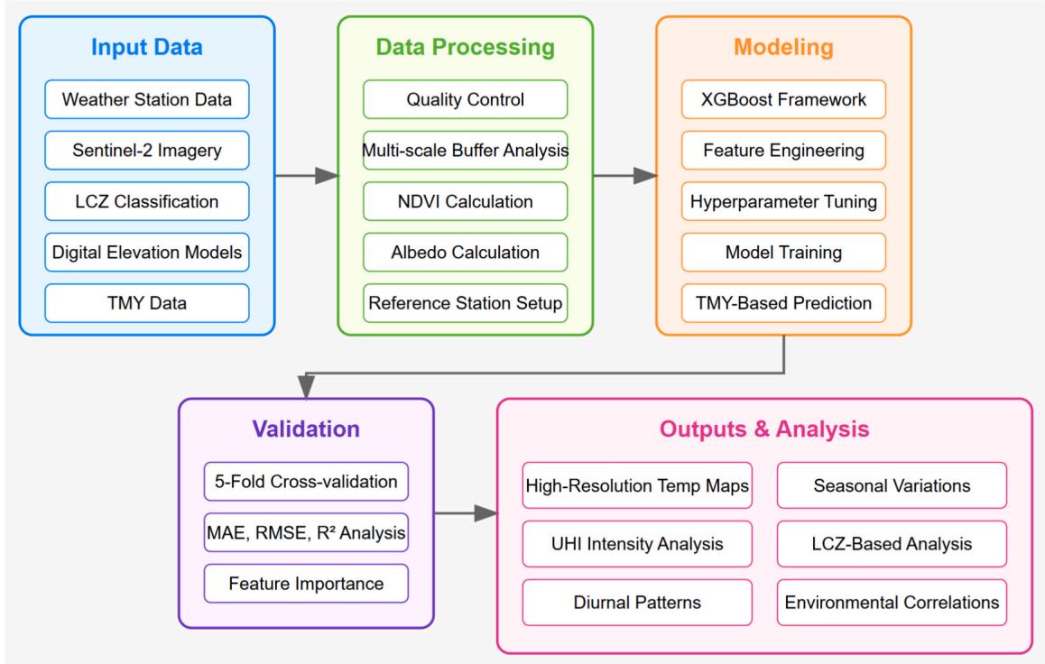Fig. 1. Urban microclimate mapping methodological framework.

complicates these conditions further, since local wind patterns and heat distribution are also influenced by the city's location close to the coast.

3.3. Data collection and processing

3.3.1. Local weather stations

To investigate Shenzhen's urban climate patterns, we purchased and leveraged data from an extensive network of weather stations operated by the China Meteorological Administration (CMA). The network integrates both national and regional monitoring stations, each adhering to the World Meteorological Organization's (WMO) guidelines for urban weather observations. All the 67 stations are plotted in Fig. 2, together with their LCZ classifications.

Eight basic meteorological parameters measured at hourly intervals are collected and used in our analysis. As detailed in Table 2, these measurements encompass the essential elements of urban climate: precipitation, wind behavior, near surface temperature, humidity, air pressure and cloud patterns. To ensure measurement consistency, we followed standardized instrument placement protocols, including having temperature sensors placed at 2- meter height, and anemometers 10- meter above ground level. We gave priority to a comprehensive coverage of Shenzhen's heterogeneous urban landscape when choosing the stations. The obtained network shows good spatial resolution and has dense coverage in situations with complex urban geometry or pronounced urban texture changes. Their positions and distribution allow us to see the climate nuances in the most intensively developed business districts as well as more open suburban areas. We also cross- referenced each station to high resolution digital elevation models to validate the geographical accuracy of our station network.

The reliability of urban climate analysis hinges on data quality, prompting to develop a sophisticated three- phase quality control framework. In the first phase, we tackled the technical challenges of data formatting. Our custom- developed algorithms managed multiple character encodings (UTF- 8, GB2312, GB18030), standardized temporal references, and standardized all timestamps to Beijing time $(\mathrm{UTC} + 8)$ . This standardization proved crucial for maintaining data consistency across the network. The second phase focused on data validation, where we employed context- based thresholds to identify anomalous readings. Rather than applying rigid criteria, we considered the local climate context and seasonal patterns when evaluating measurement validity. This approach helped distinguish between extreme events and instrumental errors. Our data completeness assessment formed the third quality control phase. Through careful analysis of temporal patterns, we identified stations with significant data gaps. To maintain the highest standards of data integrity, we excluded stations showing more than $20\%$ missing data in any given month. For the remaining stations, we achieved $98.2\%$ temporal completeness across the study period (2017 through 2021). We also deliberately preserved longer gaps as missing values to avoid introducing artificial patterns into the dataset.

3.3.2. Environmental integration of remote sensing data

Urban temperature patterns are strongly influenced by their surrounding environmental context. To comprehensively characterize these influences, we integrated four key environmental factors: urban morphology through LCZ classification, vegetation and surface properties from Sentinel- 2 imagery, and topographic characteristics from digital elevation models. Each factor was selected based on its established relationship with urban heat patterns and local climate modification.

The LCZ classification, following the WUDAPT protocol [55], provided a standardized framework for characterizing urban morphology. This classification is crucial as building density, height, and arrangement significantly affects local air flow, radiation balance, and heat storage capacity. For each weather station, we calculated the proportion of each LCZ class within multiple circular buffers $(500~\mathrm{m})$ to $3000~\mathrm{m}$ using the equation provided in Appendix A1 (Equation A(1)).

Vegetation and surface albedo significantly modify local energy balance through evapotranspiration and radiation reflection. We processed Sentinel- 2 Level- 2A imagery from 2020 using Google Earth

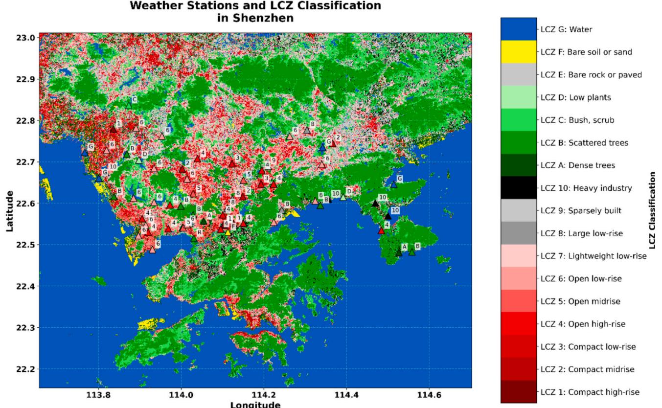
Fig. 2. The local weather stations with their LCZ information.

Table 2 Summary of weather variables measured by the automatic weather station network in Shenzhen.

Engine (GEE) to derive these parameters [56]. The Normalized Difference Vegetation Index (NDVI) [57] was calculated as described in Appendix A1 (Equation A(2)). Cloud masking was implemented using the QA60 band, with pixels flagged as clouds or cirrus being excluded from the analysis. High NDVI values indicate dense vegetation, which can significantly reduce local temperatures through increased evapotranspiration and shading.

Surface albedo $(\alpha)$ , a key parameter in urban radiation balance [58], was computed through a weighted combination of Sentinel- 2 bands (see Equation A(3) in Appendix A1).The coefficients in the equation were optimized to account for the varying contributions of different wavelengths to total solar reflection. The mean NDVI and albedo calculation results in 2020 for Shenzhen are shown Fig. 3.

Topographic effects on temperature were characterized using highresolution Digital Elevation Models (DEMs) [59]. For each location, we computed both absolute elevation and relative terrain parameters within multiple buffer zones. Local terrain roughness $(R_{t})$ which influences air flow and cold air drainage, was calculated using the method detailed in Appendix A2 (Equation A(4)- A(6)).

The GEE processing workflow we have adopted can ensure data quality through multiple steps. For Sentinel- 2 data, we filtered images with cloud coverage below $20\%$ and applied rigorous atmospheric correction. The QA60 band was used to mask residual clouds and shadows. DEM processing included void filling and edge artifact removal to ensure continuous coverage of the study area. All environmental parameters were computed at 10- meter resolution to capture fine- scale urban variability. This multi- scale approach allows us to capture both local and neighborhood- scale environmental influences on urban temperature. The visualization of the calculated elevation data for Shenzhen is illustrated in Fig. 4.

The integration of these environmental parameters revealed Shenzhen's complex urban- environmental gradients. NDVI values ranged from 0.15 in dense urban cores to 0.85 in peripheral forests, while surface albedo varied from 0.10 to 0.25. Elevation gradients showed significant variation $(0 - 943\mathrm{m})$ , creating distinct topo climatic zones. These patterns closely aligned with LCZ classifications, highlighting the interconnected nature of urban form, vegetation, and topography in shaping the local climate conditions of Shenzhen.

3.4. Reference station-based temperature mapping

The high- resolution urban temperature mapping methodology we developed employs a reference station framework that leverages the relationship between a carefully selected reference weather station and the broader urban air temperature field. This approach enables the development of a robust spatial- temporal temperature prediction model while minimizing the impact of temporal meteorological variations.

The reference station selection follows three primary criteria: (1) data completeness and quality, (2) temporal coverage alignment with TMY data, which means that the reference station is one of the stations where the TMY weather data of the specific city is generated. For a candidate station to be considered as reference, its temporal completeness must exceed $98\%$ with a maximum of 3- hour continuous missing data gaps, which can be addressed through linear interpolation:

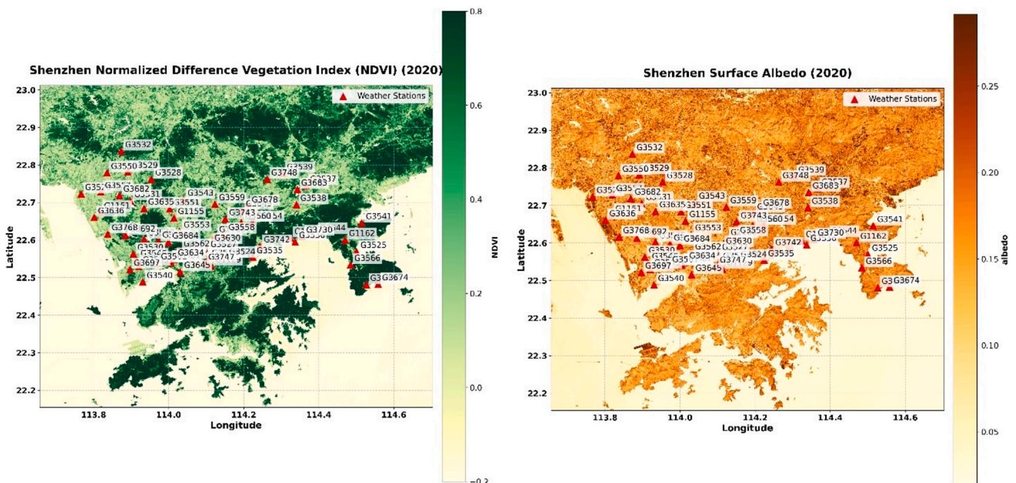
Fig. 3. Visualization of NDVI and albedo in Shenzhen calculated by Google Earth Engine.

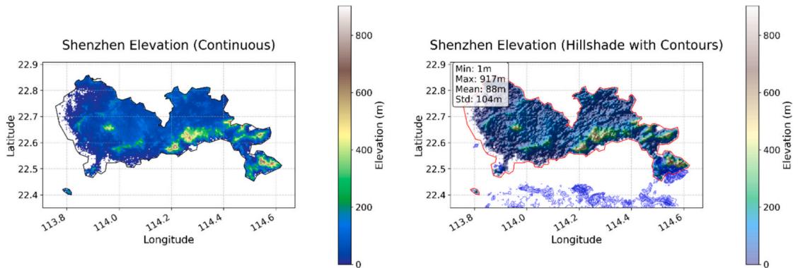
Fig. 4. Visualization of elevation data in Shenzhen.

$$T_{missing} = T_{1} + \frac{t - t_{1}}{t_{2} - t_{1}} (T_{2} - T_{1})$$

where $T_{missing}$ is the interpolated temperature, $T_{1}$ and $T_{2}$ are temperatures at times $t_{1}$ and $t_{2}$ respectively. The reference station used in this study for Shenzhen's air temperature modeling and mapping is the Bao'an International Airport station. The reference station framework establishes a baseline temperature field $T_{b}(x,y,t)$ through the relationship:

$$T_{b}(x,y,t) = T_{r}(t) + \Delta T(x,y,t)$$

where $T_{r}(t)$ represents the reference station temperature at time $t$ , and $\Delta T(x,y,t)$ denotes the temperature difference field between any location $(x,y)$ and the reference station. This framework enables the separation of temporal and spatial components in temperature variation. The validation of reference station performance utilizes a cross- validation strategy based on groupwise data splitting, ensuring temporal consistency in the validation process. For each validation fold, we calculate the Mean Absolute Error (MAE) and Root Mean Square Error (RMSE) as validation metrics, which are detailed in Appendix A4 (Equations (A10) and (A11)).

The proposed framework's effectiveness is evaluated through both spatial and temporal analyses later in the modeling procedure. Spatially, we assess the model's ability to capture temperature variations across different urban morphologies and land cover types. Temporally, we examine the framework's performance across different times of day and seasons, with particular attention to extreme temperature events and UHI intensification periods.

3.5. Data-driven model development and validation

The gradient boosting framework based on XGBoost [60] is employed to predict high resolution urban temperature fields using the temperature mapping algorithm. Considering the potential application of other machine learning approaches including Random Forest (RF), Deep Learning (DL), and Geographically Weighted Regression (GWR), we selected XGBoost for this study based on several key considerations:

• Data Compatibility: XGBoost can efficiently handle both continuous environmental variables and categorical features without extensive preprocessing.- Interpretability: Unlike "black box" models, XGBoost provides interpretable feature importance metrics crucial for urban planning applications.- Performance with Limited Data: XGBoost shows superior performance with moderate-sized datasets typical in urban climate studies where weather station networks are inherently limited.

• Computational Efficiency: Compared to GWR, XGBoost can capture non-linear spatial relationships more efficiently while maintaining lower computational requirements.- Non-linear Relationship Modeling: XGBoost can effectively capture complex relationships between urban form and temperature without assuming spatial stationarity (a limitation of standard GWR).

While RF has been successfully applied in similar contexts [32], XGBoost's regularization parameters can offer better control over model complexity for spatiotemporal prediction tasks in heterogeneous urban environments. Spatially and temporally continuous temperature predictions are generated through this approach by combining the so- called static environmental features with dynamic meteorological conditions from the reference station. The algorithm's feature space consists of two primary components: static environmental characteristics $(X_{s})$ and dynamic meteorological variables $(X_{d})$ . For any location $(x,y)$ at time $t$ , the temperature prediction is formulated as:

$$T(x,y,t) = f(X_{s}(x,y),X_{d}(t)) + \epsilon$$

where $f$ represents the XGBoost model and $\epsilon$ denotes the prediction error. The static features $X_{s}$ incorporate multi- scale environmental parameters obtained through buffer analysis at radii ranging from $500\mathrm{m}$ to $3000\mathrm{m}$ :

$$X_{s} = \{X_{LCZ},X_{NDVI},X_{albedo},X_{elev}\}$$

where $X_{LCZ}$ represents LCZ classifications, $X_{NDVI}$ captures vegetation indices, $X_{albedo}$ describes surface reflectance properties, and $X_{elev}$ accounts for terrain characteristics.

Dynamic features $X_{d}$ from the reference station include:

$$X_{d} = \{T_{r},RH_{r},P_{r},W_{s},W_{d},t_{month},t_{hour}\}$$

where (T_{r},RH_{r},P_{r},W_{s},W_{d},t_{month},t_{hour}}) where (T_{r},RH_{r},P_{r},W_{s},W_{d},t_{month},t_{hour}}) where (T_{d},RH_{d},P_{d},W_{s},W_{d},t_{month},t_{hour})) represent temperature, relative humidity, and pressure respectively; (W_{s}) and (W_{d}) denote wind speed and direction; and (t_{month},t_{hour}) capture temporal patterns.

The XGBoost model optimizes an ensemble of decision trees through gradient boosting (see Equation (A12) in Appendix A). The model minimizes an objective function that balances prediction accuracy with model complexity, as detailed in Appendix A3 (Equations A(7)- A(9)). Model hyperparameters are optimized through Bayesian optimization [61] using the search space present in Table 3.

Model validation employs a comprehensive testing strategy that evaluates prediction accuracy using multiple metrics. The primary evaluation metrics include MAE, RMSE, and coefficient of determination $(R^{2})$ , calculated as detailed in Appendix A4 (Equations ((A10)- (A12)).

In this research, feature importance is tested using both model- based metrics and permutation tests to ensure robust feature selection. For XGBoost model training, we prevent model overfitting while keep predictive accuracy using early stopping with a patience of 50 rounds.

Table 3 Hyperparameter ranges for XGBoost model optimization.

Station- wise performance analysis is used to assess how well the final model performs on an independent test set, and insights are provided regarding spatial prediction reliability. To account for potential scale differences in features, all input variables undergo data standardization as follows:

$$X_{scaled} = \frac{X - \mu_X}{\sigma_X}$$

where $\mu_{X}$ and $\sigma_{X}$ represent the mean and standard deviation of feature X respectively, calculated from the training data.

We then used the model to generate high resolution spatiotemporal air temperature maps using the TMY data as reference inputs and post process to validate it with historical weather station data. This approach was chosen for several reasons. TMY data is based on typical weather conditions calculated from multiple years of long- term meteorological observations and is more reliable than any single year for analyzing characteristic urban temperature patterns. Our results can be easily applicable to practical urban planning and building energy analysis because TMY data is popular in urban and building design applications. In addition, the use of TMY data guarantees consistent temporal coverage and removes variability due to missing data or anomalous weather events in the historical records.

The high- resolution temperature mapping procedure consists of four main steps. The first step involves spatial grid generation, where we create a regular $500\mathrm{m}\times 500\mathrm{m}$ grid covering the entire study area. These grid cells are clipped to the administrative boundary of Shenzhen, with the cell size selection carefully balancing computational efficiency with spatial resolution requirements. In the second step, we perform environmental feature extraction for each grid cell, calculating static environmental features according to the equation $X_{s} =$ $f(LCZ_{r},NDVI_{r},\alpha_{r},z)$ ,where r represents different buffer radii $500~\mathrm{m}$ $5000\mathrm{m})$ ,and $\mathbb{Z}$ is elevation. These features are calculated through buffer analysis centered on each grid cell, with all remote sensing data (LCZ, NDVI, albedo) resampled to match the grid resolution. The third step encompasses temperature prediction, where for each hour in the TMY dataset, we calculate $T(x,y,t) = f(X_{s}(x,y),X_{d}(t))$ ,where $X_{d}(t)$ represents dynamic variables from TMY data. The grid system meshed for Shenzhen is plotted in Fig. 5, resulting in a total number of 7610 cells.

Then, all grid cells will be predicted simultaneously, and the results are stored in a structured netCDF format for efficient data handling [62]. The last step is visualization and analysis in which temperature distributions are visualized with consistent color scale. Spatial interpolation is done where needed by bilinear methods and results are masked to the administrative boundary. These high- resolution temperature predictions are then used to perform the subsequent UHI analysis. The UHI of a location $(\mathbf{x},\mathbf{y})$ at a time t is the temperature deviation from the spatial mean.

3.6.UHI pattern analysis

The UHI analysis employs a comprehensive framework to characterize spatial patterns and temporal evolution of urban temperature anomalies. The UHI at any location $(\mathbf{x},\mathbf{y})$ and time t is quantified as the temperature deviation from rural reference temperature:

$$UHI(x,y,t) = T(x,y,t) - T_{rural}(t)$$

where $\mathrm{T(x,y,t)}$ denotes the predicted temperature at location $(\mathbf{x},\mathbf{y})$ and time t, and $T_{rural}(t)$ represents the mean temperature of rural areas at time t. Rural areas are defined as locations classified as Local Climate Zones (LCZ) 11- 17, which represent natural and non- urban landscapes including dense trees, scattered trees, bush/scrub, low plants, bare rock/ paved surfaces, bare soil/sand, and water bodies.

The temporal decomposition of UHI patterns is conducted through diurnal and seasonal analyses. The mean diurnal UHI for hour h is calculated separately for each LCZ class:

$$UHI_{h}(LCZ) = \frac{1}{N_{LCZ}}\sum_{i = 1}^{N_{LCZ}}UHI(x_{i},y_{i},t_{h})$$

where $N_{LCZ}$ represents the number of grid cells within each LCZ class, and $t_h$ denotes the time at hour h.

For seasonal analysis, the monthly mean UHI is computed for each

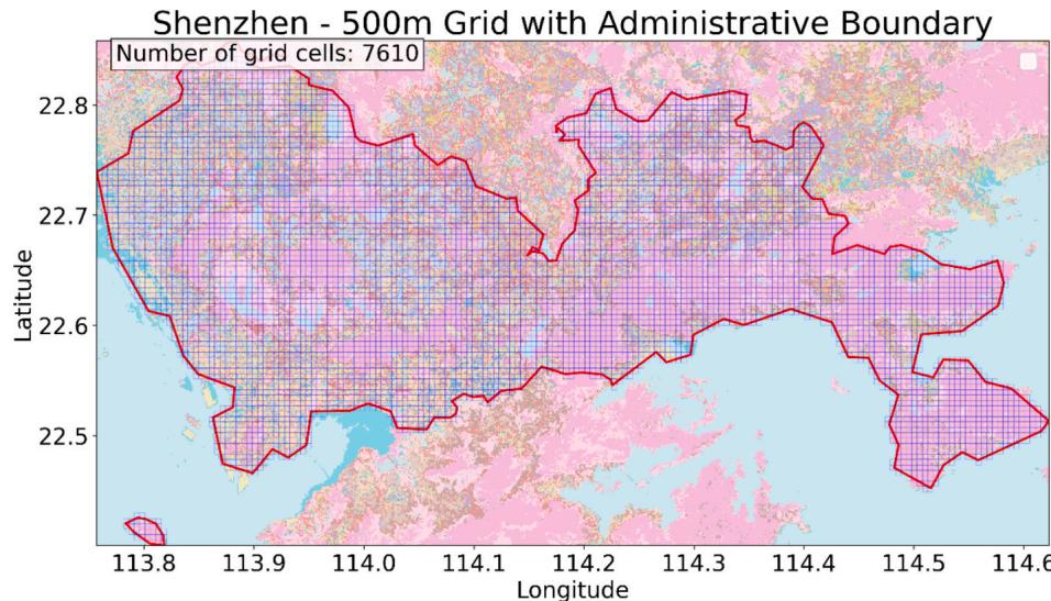
Fig. 5. Grid system meshed for Shenzhen's administrative boundary.

LCZ:

$$U H I_{m}(L C Z) = \frac{1}{N_{L C Z}H_{m}}\sum_{i = 1}^{N_{L C Z}}\sum_{i\in m}U H I(x_{i},y_{i},t)$$

where $H_{m}$ represents the total number of hours in month m.

The analysis also distinguishes between daytime (06:00- 18:00) and nighttime (18:00- 06:00) UHI patterns, as well as seasonal variations between summer (June- August) and winter (December- February) months to capture the temporal dynamics of the urban thermal environment.

To identify persistent hot spots and cool islands, we employ a threshold- based classification:

$$\begin{array}{rl} & {Z_{hot}(x,y) = \left\{ \begin{array}{ll}1 & {\mathrm{if}\overline{UHI} (x,y) > \mu +\sigma}\\ 0 & {\mathrm{otherwise}} \end{array} \right.}\\ & {Z_{cool}(x,y) = \left\{ \begin{array}{ll}1 & {\mathrm{if}\overline{UHI} (x,y)< \mu -\sigma}\\ 0 & {\mathrm{otherwise}} \end{array} \right.} \end{array}$$

where $\overline{UHI} (x,y)$ is the time- averaged UHI, $\mu$ and $\sigma$ are the spatial mean and standard deviation of $\overline{UHI}$ respectively.

The relationship between UHI patterns and environmental factors is analyzed through LCZ stratification. For each LCZ class $k_{i}$ the characteristic UHI is calculated as:

$$U H I_{L C Z_{k}} = \frac{1}{N_{k}}\sum_{(x,y)\in L C Z_{k}}\overline{{U H I}} (x,y)$$

where $N_{k}$ is the number of grid cells belonging to LCZ class $\mathbf{k}$

4.Results

4.1. Model performance analysis

4.1.1.Cross-validation results

The XGBoost model's performance was evaluated through a comprehensive five- fold cross- validation framework, incorporating both spatial and temporal validation strategies. The distribution of Mean Absolute Error (MAE) across the five folds shows a gradual improvement from Fold 1 to Fold 5 as shown in Fig. 6, with median MAE values ranging from $0.71^{\circ}\mathrm{C}$ in the first fold to $0.56^{\circ}\mathrm{C}$ in the final fold. The interquartile ranges remain relatively stable across folds, indicating consistent model performance. The overall cross- validation MAE of $0.56^{\circ}\mathrm{C}$ suggests a strong predictive capability, with $90\%$ of predictions falling within $\pm 0.85^{\circ}\mathrm{C}$ of observed values. The XGBoost model's performance (MAE: $0.56^{\circ}\mathrm{C}$ ) demonstrates robust predictive capability that surpasses comparable approaches such as Chen et al. (MAE: $0.89^{\circ}\mathrm{C}$ ) [32] and Zhang et al. (MAE: $0.72^{\circ}\mathrm{C}$ ) [34]. This improvement likely stems from our integration of multi- scale environmental parameters, which captures urban complexity more effectively than single- scale analyses. The superior performance in urban core areas (MAE: $0.34 - 0.40^{\circ}\mathrm{C}$ ) compared to peripheral regions (MAE: $0.53 - 0.57^{\circ}\mathrm{C}$ ) reveals the model's sensitivity to urban form complexity and suggests that urban morphological features provide stronger predictive signals than natural landscapes.

Fig. 7 shows the model's performance using scatter plot analysis, which indicates good correlation between predicted and observed temperatures for both training and test set. On the training set $(n = 740,123)$ the model has an $\mathbb{R}^2$ of 0.995 and MAE of $0.27^{\circ}\mathrm{C}$ , and is robust on the test set $(n = 189,544)$ with an $\mathrm{R}^2$ of 0.980 and MAE of $0.56^{\circ}\mathrm{C}$ . This small degradation in performance between training and testing scenarios indicates effective model generalization and a low level of overfitting. Fig. 8 also shows temporal validation results with good model performance across varying seasons and urban contexts. Summer predictions at stations in urban and outskirt areas are strong predictors, with $\mathbb{R}^2$ values in the range of 0.791- 0.915. During the summer months, the model effectively captures the diurnal temperature pattern at stations G3566 (Nan'ao Harbor, $\mathrm{MAE} = 0.57^{\circ}\mathrm{C}$ ) and G3166 (Buji, $\mathrm{MAE} = 0.40^{\circ}\mathrm{C}$ ). Similar robust performance is shown with winter predictions also, where $\mathbb{R}^2$ values $>0.90$ at all validated stations and MAE values of $0.34^{\circ}\mathrm{C}$ to $0.76^{\circ}\mathrm{C}$ .

In core urban areas, the model shows slightly better performance than in peripheral regions, probably because the urban fabric in central areas is more uniform and the station network is denser. Nevertheless, the performances show little differences, with MAE variations below $0.3^{\circ}\mathrm{C}$ between urban and peripheral stations. Temporal analysis shows that model performance is decent during winter months with about $15\%$ lower average MAE than summer predictions. The reduced accuracy during winter is attributed to the addition of seasonal variation due to more stable atmospheric conditions and less convective activity during winter. The model reproduces both the magnitude and timing of diurnal temperature cycles well and is particularly good at reproducing diurnal cycles at night, which might be the time of greatest UHI effect as shown in previous studies [24]. Results of model validation indicate the robust ability of the model to predict urban temperatures on a variety of spatial and temporal scales in order to provide a reliable basis from which to analyze future urban climates.

4.1.2. Feature importance

In this research, feature importance analysis was conducted through two complementary approaches - correlation analysis and permutation

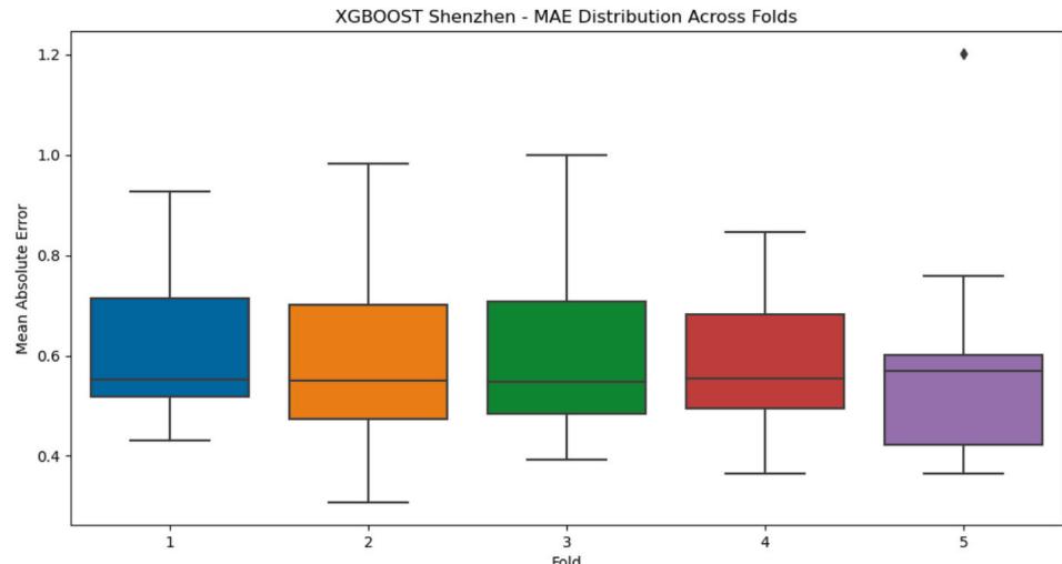
Fig. 6. Five-fold cross-validation results of the XGBoost model.

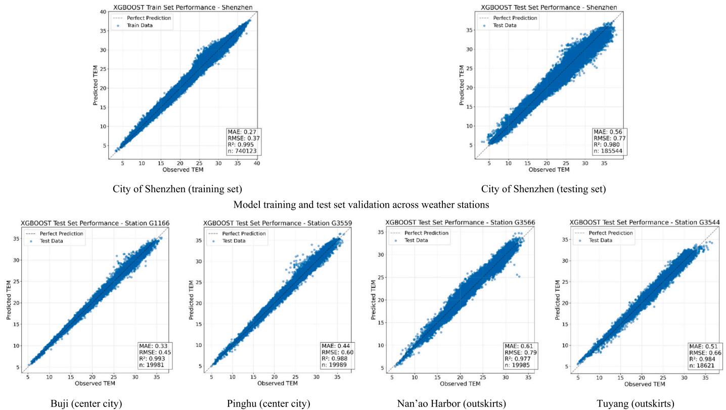
Fig. 7. Scatter plots of XGBoost model validation of the whole city and random weather station.

importance testing. The correlation analysis reveals distinct patterns among environmental features across different spatial scales, and its results are shown in Fig. 9.

LCZ features exhibit strong internal correlations $(\mathrm{r} > 0.90)$ at adjacent spatial scales, with correlation strength gradually decreasing as the distance between scales increases. This pattern reveals the multi- scale nature of urban morphological influences on temperature, suggesting that urban form affects thermal conditions through nested spatial hierarchies rather than at distinct, separate scales. The diminishing correlation strength at larger distances indicates a spatial threshold beyond which new environmental information becomes increasingly independent from local conditions, challenging the notion that urban climate is primarily determined by immediate surroundings.

NDVI features also show similar scale- dependent correlations but with a more rapid decay in correlation strength beyond $2000~\mathrm{m}$ buffers. Albedo features demonstrate moderate to strong correlations $(\mathbf{r} =$ 0.60- 0.95) across different scales, indicating more gradual changes in surface reflectance properties.

Dynamic meteorological variables display expected physical relationships, with significant correlations observed between temperature (TEM) and relative humidity (RHU) $(\mathrm{r} = 0.22)$ , and between wind speed (WIN_S_Avg_2mi) and direction (WIN_D_Avg_2mi) $(\mathrm{r} = 0.24)$ . Notably, pressure (PRS) shows strong negative correlation with temperature $(\mathbf{r} =$ - 0.79), reflecting the typical atmospheric relationship in urban environments.

The permutation importance analysis quantifies each feature's contribution by measuring the decrease in model performance when the feature values are randomly permuted, and its results are shown in Fig. 10. More negative values indicate greater importance, as they represent larger degradation in model performance when that feature is randomized. The analysis reveals the following hierarchical influences of static features are the five most important factors:

1. LCZ classification at $1000~\mathrm{m}$ radius 2. Surface albedo at $1000~\mathrm{m}$ radius

3. LCZ classification at $1500~\mathrm{m}$ radius
4. Surface albedo at $1500~\mathrm{m}$ radius
5. Surface albedo at $3000~\mathrm{m}$ radius

Moreover, dynamic meteorological variables show larger decreases in model performance, particularly pressure (PRS, $- 0.15$ ) and reference air temperature (TEM, $- 0.14$ ), indicating their crucial role as baseline predictors. However, the relatively smaller decreases in performance for urban surface characteristics suggest they provide essential fine- scale spatial information that complements the meteorological variables. The combined analysis of correlation patterns and permutation importance reveals a complex interplay between features at different spatial scales. While meteorological variables provide the fundamental basis for temperature prediction, the urban surface characteristics at multiple scales $(500\mathrm{m - }3000\mathrm{m})$ can contribute to critical spatial detail necessary for high- resolution temperature mapping.

4.2. Temperature distribution patterns

4.2.1. Spatial characteristics

The high- resolution temperature mapping reveals distinct spatial patterns of temperature distribution across Shenzhen's urban landscape as shown in Fig. 11. During a representative winter day (January 3, 13:00), the temperature varies considerably across the city, ranging from $19.17^{\circ}\mathrm{C}$ to $23.61^{\circ}\mathrm{C}$ with a mean of $21.31^{\circ}\mathrm{C}$ . The $4.44^{\circ}\mathrm{C}$ temperature range $(19.17^{\circ}\mathrm{C}$ to $23.61^{\circ}\mathrm{C})$ observed during a representative winter day reveals the profound influence of urbanization on Shenzhen's thermal environment. This magnitude of intra- urban temperature variation—equivalent to the warming effect expected from several decades of global climate change—underscores how urban development creates distinct microclimates that may amplify or offset larger climate trends. The persistence of this thermal pattern in summer, despite different atmospheric conditions, suggests that urban structure rather than seasonal weather processes is the dominant driver of Shenzhen's spatial temperature distribution.

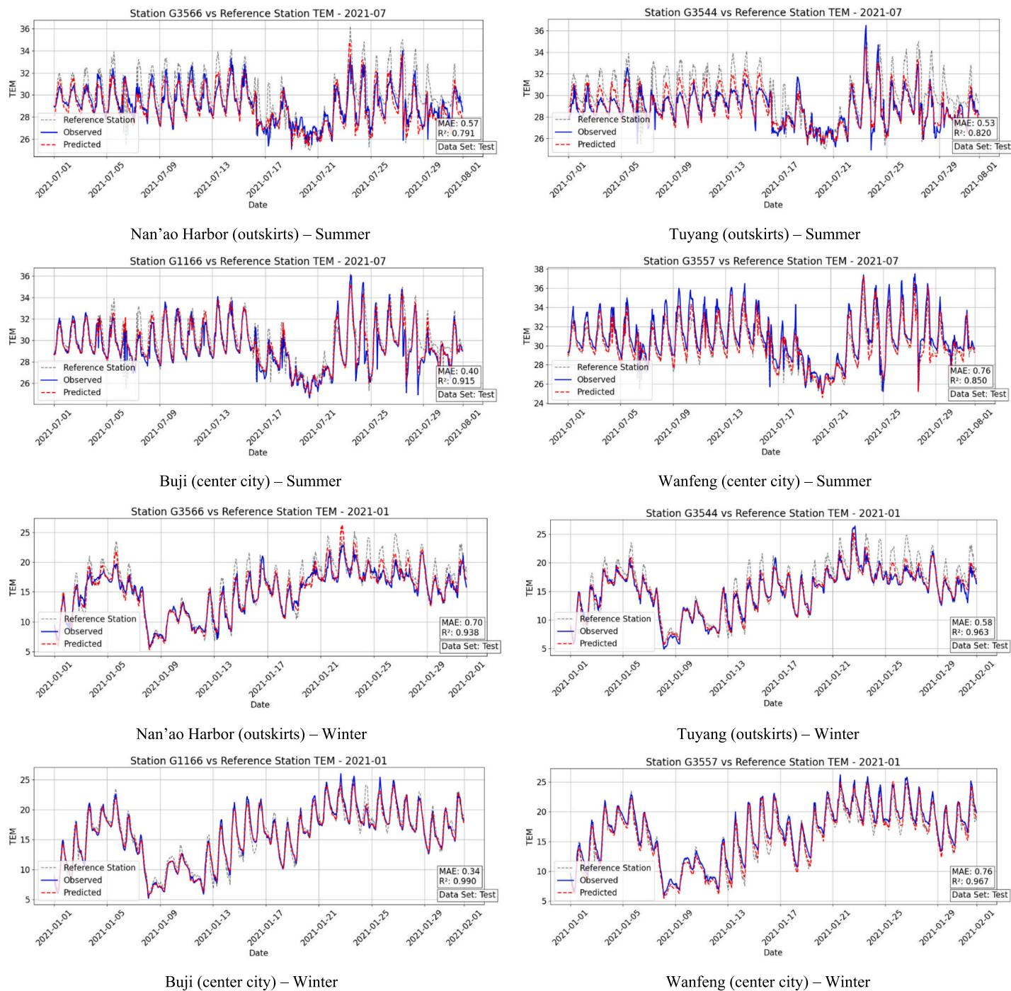
Fig. 8. Time series plots of XGBoost model validation of sample weather stations in representative months of summer and winter.

The western region of Shenzhen, particularly around coordinates $(113.9^{\circ}\mathrm{E}, 22.7^{\circ}\mathrm{N})$ , exhibits notably higher temperatures, forming a prominent warm core with temperatures exceeding $22.24^{\circ}\mathrm{C}$ . This thermal pattern likely reflects the intense urban development and human activities in this area. The summer temperature distribution, captured on August 1 at 13:00, demonstrates even more pronounced spatial variability. The temperature range extends from $28.52^{\circ}\mathrm{C}$ to $33.89^{\circ}\mathrm{C}$ , with a mean of $31.38^{\circ}\mathrm{C}$ . Interestingly, the spatial pattern of elevated temperatures shows remarkable consistency with the winter distribution, suggesting persistent structural influences on urban temperature patterns. The western urban core consistently maintains higher temperatures, with values reaching above $33.16^{\circ}\mathrm{C}$ during peak summer conditions.

Further analysis of these temperature patterns reveals the presence of distinct urban heat and cool islands throughout Shenzhen, as illustrated in Fig. 12. The western portion of the city is characterized by significant UHI formations, depicted in red, indicating areas of persistent elevated temperatures. In contrast, the eastern regions, particularly around coordinates $(114.4^{\circ}\mathrm{E}, 22.6^{\circ}\mathrm{N})$ , display notable urban cool islands, shown in blue. This east- west thermal gradient appears to be a defining feature of Shenzhen's urban microclimate structure.

The spatial distribution of these thermal patterns demonstrates a strong correlation with the city's urban morphology and development intensity. UHI's predominantly coincide with areas of dense urban development and commercial activity in the western districts, while cool islands are more prevalent in the eastern regions where urban density is generally lower and green spaces are more abundant. The temperature gradient shows a clear urban- rural transition, with temperature differences of up to $4.44^{\circ}\mathrm{C}$ in winter and $5.18^{\circ}\mathrm{C}$ in summer between the urban core and peripheral areas. The high- resolution mapping also

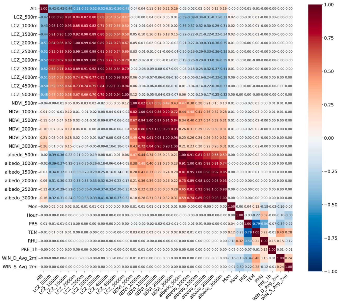
Fig. 9. Feature correlation analysis.

reveals several localized thermal features, including small- scale heat pockets and cool spots, that would be missed by traditional lower- resolution temperature monitoring approaches. These microscale variations in urban temperature highlight the complex interplay between built environment characteristics and local climate conditions, underscoring the importance of high- resolution temperature mapping for urban climate research and planning applications.

We have summarized the urban heat and cool islands in Shenzhen in Table 4. Quantitative analysis of the thermal zones provides further insights into the distribution of urban heat patterns. It can be seen that UHIs occupy $10.00\%$ of the study area, comprising 718 grid cells with a mean temperature elevation of $0.60^{\circ}\mathrm{C}$ above the city average. The majority of the city $(79.99\%)$ 6,742 grid cells) falls within the neutral zone, showing minimal temperature deviation $(- 0.01^{\circ}\mathrm{C})$ from the mean. Urban cool islands account for $10.01\%$ of the area with 719 grid cells, exhibiting an average temperature depression of $0.53^{\circ}\mathrm{C}$ below the city mean. This balanced distribution of heat and cool islands suggests a complex urban thermal structure that reflects the diverse urban landscape of Shenzhen.

4.2.2. Temporal variations

As shown in Fig. 13, the temporal analysis of Shenzhen's UHI effect reveals distinct patterns across different time scales. The diurnal variation, illustrated in Fig. 13 (left), demonstrates a clear day- night cycle in UHII. The mean UHII is lowest (approximately $0^{\circ}\mathrm{C}$ ) during early morning hours (around 4:00- 6:00) and increases significantly during the day, reaching its peak of about $0.5^{\circ}\mathrm{C}$ in the early afternoon (around 14:00- 15:00). Following this peak, the UHII gradually decreases through the evening and night hours. The shaded area, representing the variation range of UHII, shows considerable spread throughout the 24- hour cycle, with the largest variations occurring during the afternoon hours when the mean UHI is strongest.

The seasonal pattern (Fig. 13, right) indicates a relatively consistent mean UHII throughout the year, with values generally ranging between $0.2^{\circ}\mathrm{C}$ and $0.4^{\circ}\mathrm{C}$ . There is a slight increase in UHII during the warmer months (around months 6- 8, corresponding to summer), where the mean intensity reaches approximately $0.35^{\circ}\mathrm{C}$ . The variation range (shown by the blue shaded area) remains fairly consistent across all months, suggesting that the spatial heterogeneity of the UHI effect is relatively stable seasonally, despite small changes in mean intensity. This seasonal variation is further elaborated through the detailed LCZ

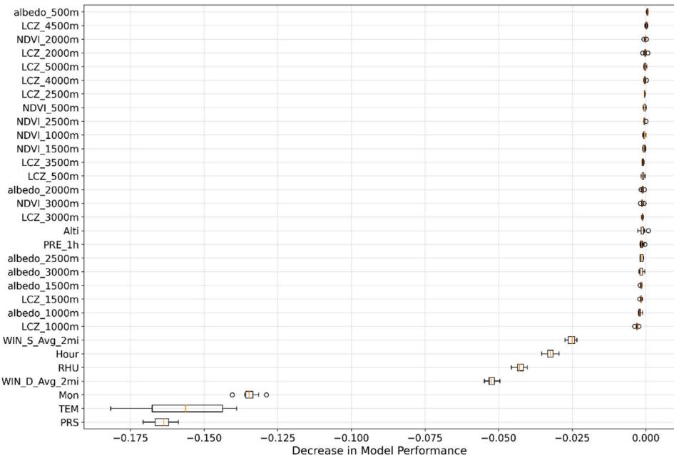
Fig. 10. Feature permutation importance analysis.

analysis presented in Fig. 14.

The LCZ- based seasonal analysis reveals complex temporal patterns across different urban morphologies. Compact high- rise areas (LCZ 1) consistently show the strongest UHI effect throughout the year, with intensity peaks reaching $0.97^{\circ}\mathrm{C}$ in July and maintaining relatively high values $(0.82 - 0.88^{\circ}\mathrm{C})$ during the summer months (April- September). Similarly, open high- rise zones (LCZ 4) display strong but slightly moderated UHI intensities, with values ranging from $0.75 - 0.87^{\circ}\mathrm{C}$ during summer months. In contrast, areas with dense trees (LCZ 11) consistently demonstrate a cooling effect, showing negative UHI intensities throughout the year, with values ranging from $- 0.19^{\circ}\mathrm{C}$ to $- 0.05^{\circ}\mathrm{C}$ , with the strongest cooling effect observed in May. Industrial areas (LCZ 10) exhibit a relatively strong UHI effect with a distinct peak in November $(0.75^{\circ}\mathrm{C})$ , showing notably higher intensities compared to the summer months. Low- rise development patterns show varying degrees of UHI, with compact low- rise (LCZ 3) areas experiencing moderate UHI effects $(0.54 - 0.86^{\circ}\mathrm{C}$ during summer), while large low- rise (LCZ 8) and open low- rise (LCZ 6) areas show weaker UHI intensities (generally below $0.55^{\circ}\mathrm{C}$ ). Notably, sparsely built areas (LCZ 9) demonstrate remarkably stable UHI intensities throughout the year, varying only between $0.22 - 0.42^{\circ}\mathrm{C}$ . Natural surfaces show distinct patterns: low plants (LCZ 14) exhibit moderate UHI intensities $(0.36 - 0.41^{\circ}\mathrm{C}$ in summer), while bare rock/paved surfaces (LCZ 15) and bare soil/sand (LCZ 16) show relatively strong UHI effects, particularly during summer months, with values reaching $0.68^{\circ}\mathrm{C}$ and $0.62^{\circ}\mathrm{C}$ respectively. Water bodies (LCZ 17) maintain moderate UHI intensities throughout the year, ranging from $0.23^{\circ}\mathrm{C}$ to $0.56^{\circ}\mathrm{C}$ . This analysis reveals a maximum seasonal variation of $1.16^{\circ}\mathrm{C}$ and a summer- winter contrast of $0.27^{\circ}\mathrm{C}$ across all LCZ types, highlighting the significant influence of urban morphology on the seasonal dynamics of Shenzhen's thermal environment.

4.3. UHI pattern analysis

4.3.1. Intensity distribution

Fig. 15 plots the spatial distribution of UHI across Shenzhen and shows complex pattern of air temperature variations, with marked contrast between the west and east parts of the city. Variations of the annual mean values encompassing both spatial and temporal variability suggest thermal heterogeneity within the urban environment of

Shenzhen. The western part of Shenzhen, centered on coordinates $(113.8^{\circ} - 114.0^{\circ}\mathrm{E}; 22.5^{\circ}\mathrm{N} - 22.6^{\circ}\mathrm{N})$ , has the largest UHI effect, with mean UHI intensities surpassing $0.8^{\circ}\mathrm{C}$ . Multiple hot cores (defined as $\mathrm{UHII} > 1.0^{\circ}\mathrm{C}$ ) are present in this area and clustered with areas of intense urbanization.

In contrast, the UHI is less remarkable in the eastern portions of the city, especially beyond $114.3^{\circ}\mathrm{E}$ starting off the Longgang Center City, where thermal pattern is more moderate and UHI values typically vary from $- 0.25^{\circ}\mathrm{C}$ to $0.2^{\circ}\mathrm{C}$ . Notably, numerous localized cooling patches occur within the city depicted with blue patches having UHI intensities less than $- 0.4^{\circ}\mathrm{C}$ , indicating the presence of urban green space or water body. In the central portion of the city $(114.1^{\circ}\mathrm{E} - 114.2^{\circ}\mathrm{E})$ . A transitional zone of mixed thermal characteristics occurs, featuring patches of both warming and cooling effects in the heterogeneous thermal landscape. Spatial pattern also shows a clear east to west gradient of decreasing UHI with strongest UHI effect found in the west urban core. The distribution of the values is likely attributed to the city's development pattern, along with varying intensity of urbanization in different districts, where the western parts of the city experience more intense urbanization and thermal impacts.

4.3.2. Environmental factor relationships

The relationship between LCZ and UHI in Shenzhen demonstrates complex patterns across different urban morphologies and temporal scales. The diurnal analysis (Fig. 16) reveals distinct temporal signatures for different LCZ types, with three characteristic patterns emerging throughout the day. First, built- up areas (LCZ 1- 5) show a pronounced diurnal cycle with minimal UHI during early morning hours (4:00- 7:00), followed by a sharp increase starting around 8:00, reaching peak values between 13:00- 15:00. Notably, compact and open high- rise areas (LCZ 1 and LCZ 4) exhibit the most dramatic daytime intensification, reaching peak intensities of approximately $1.2^{\circ}\mathrm{C}$ during early afternoon hours in LCZ 1. Second, low- rise zones (LCZ 6- 8) display a more moderate diurnal variation, with peak intensities around $0.6 - 0.8^{\circ}\mathrm{C}$ . Third, vegetated areas, particularly those with dense trees (LCZ 11), maintain consistently lower temperatures throughout the day, showing slight negative UHI values (around $- 0.2^{\circ}\mathrm{C}$ ), demonstrating their cooling effect through shading and evapotranspiration.

The statistical distribution of UHI across different LCZs (Fig. 17) reveals clear stratification among different urban morphologies.

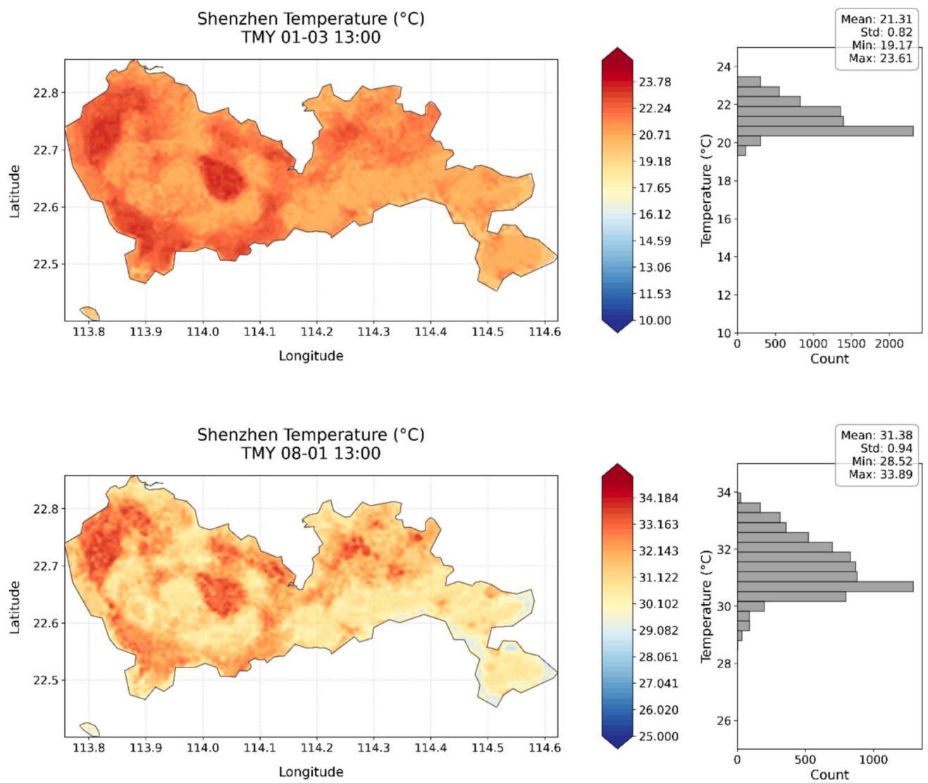
Fig. 11. High-resolution temperature mapping of representative days in winter and summer.

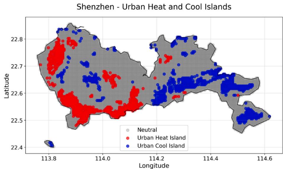
Fig. 12. Annual urban heat and cool island analysis for Shenzhen.

Table 4 Summarization of urban heat and cool islands in Shenzhen.

Compact and open high- rise zones (LCZ 1 and 4) show the highest median UHI intensities (around $0.8^{\circ}\mathrm{C}$ and large interquartile ranges, indicating both intense and variable thermal conditions. Mid- rise areas (LCZ 2- 3) show slightly lower median values $(0.6 - 0.7^{\circ}\mathrm{C})$ but maintain considerable variability. Open and large low- rise zones (LCZ 6- 8) demonstrate progressively decreasing UHI intensities, with median values ranging from $0.2 - 0.4^{\circ}\mathrm{C}$ . Natural surfaces show distinct patterns: dense trees (LCZ 11) consistently demonstrate a cooling effect with negative median UHI values (around $- 0.2^{\circ}\mathrm{C}$ ), while bare rock/paved surfaces (LCZ 15) and bare soil/sand (LCZ 16) show moderate positive UHI intensities (median values around $0.5^{\circ}\mathrm{C}$ ). Water bodies (LCZ 17) maintain intermediate UHI intensities with relatively small variability. The results highlight the strong influence of urban morphology on local thermal environments, with building height and density playing crucial roles in UHI. The clear stratification of UHI effects across different LCZs underscores the importance of urban design in mediating urban thermal comfort.

Correlation analysis results are shown in Fig. 18, which quantifies the relationships between LCZ types and UHIH across different time periods (24- hour, daytime, and nighttime), revealing significant associations between urban morphology and thermal conditions. Dense tree coverage (LCZ 11) shows the strongest negative correlation (approximately $- 0.7$ ) with UHIH across all time periods, emphasizing the crucial role of urban forestry in temperature regulation. The exceptional cooling effect of dense tree coverage (LCZ 11, $\mathrm{r} \approx - 0.7$ ) compared to scattered trees (LCZ 12, $\mathrm{r} \approx - 0.2$ ) challenges simplistic urban greening

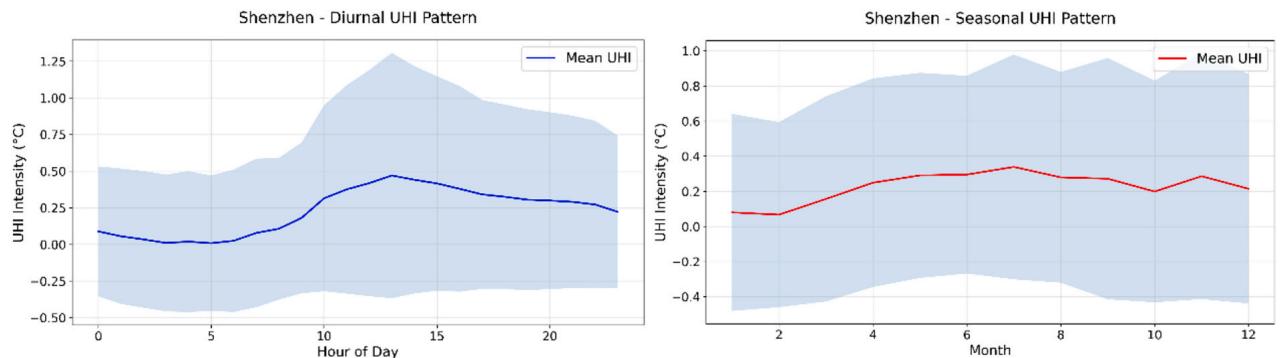
Fig. 13. Annual diurnal and seasonal patterns of mean UHIH in Shenzhen.

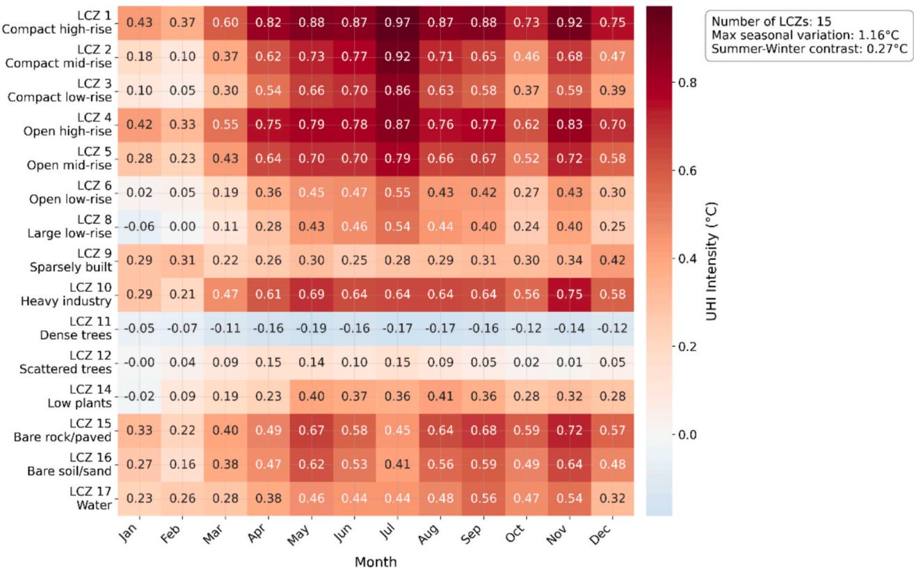
Fig. 14. Seasonal UHI patterns by LCZ in Shenzhen.

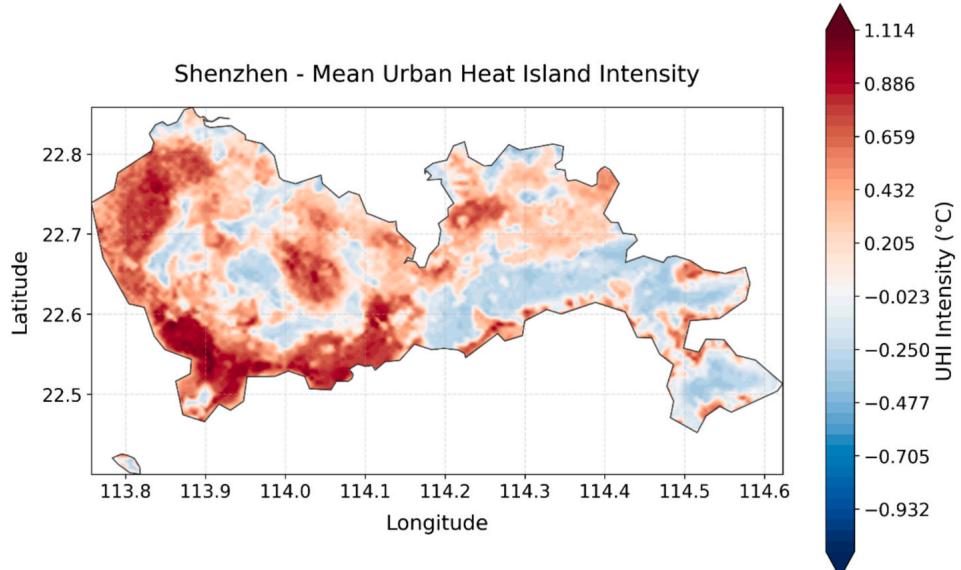
Fig. 15. Annual mean UHI distribution in Shenzhen.

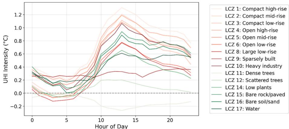Fig. 16. Diurnal UHI patterns by LCZs in Shenzhen. Shenzhen - UHI Intensity Distribution by Local Climate Zone Shenzhen - Diurnal UHI Pattern by Local Climate Zone

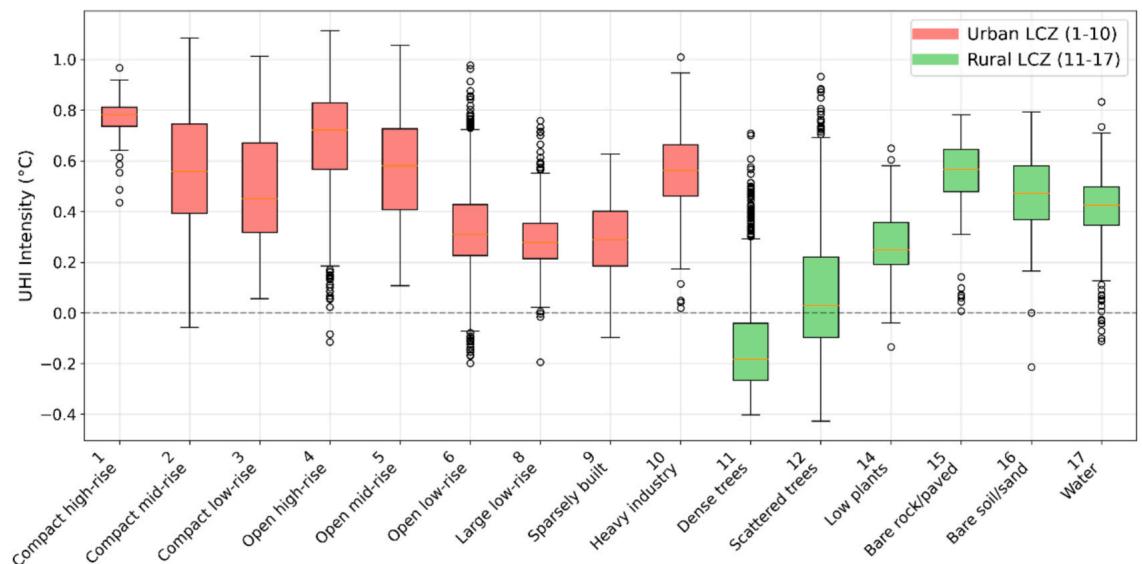Fig. 17. UHI distribution in various LCZs in Shenzhen.

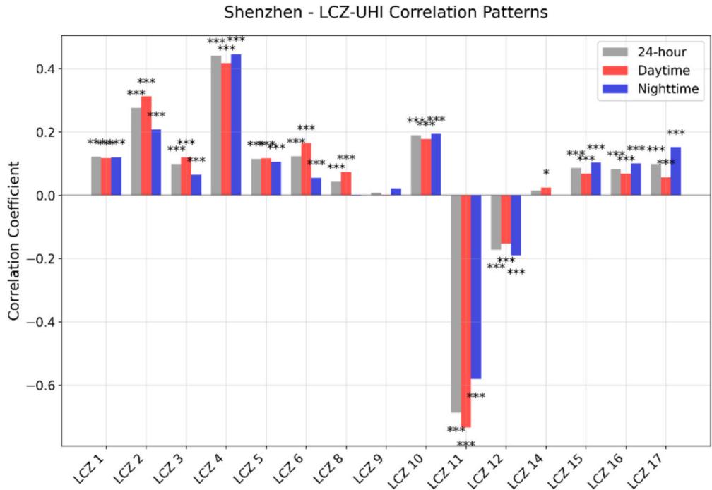
Fig. 18. Correlation analysis for LCZs and UHI relationship in Shenzhen.

approaches that focus merely on increasing tree count. This finding suggests that the spatial configuration and density of urban vegetation critically determines cooling effectiveness, with implications for optimizing urban forestry initiatives. The consistent cooling effect throughout the day may potentially be attributed to Shenzhen's subtropical climate where evapotranspiration remains active during warmer nights. Conversely, open high- rise areas (LCZ 4) exhibit the strongest positive correlation (around 0.45) for all periods, followed by compact mid- rise zones (LCZ 2) at about 0.3, indicating that vertical urban development significantly contributes to UHI formation.

The analysis reveals distinct temporal variations in these correlations. Most built- up areas (LCZ 1- 6) show statistically significant correlations $(p< 0.001)$ across all time periods, with some zones showing stronger relationships during daytime hours. For instance, compact midrise areas (LCZ 2) demonstrate a notably stronger correlation during daytime compared to nighttime (approximately 0.3 vs 0.2). Industrial areas (LCZ 10) show a consistent positive correlation (around 0.2) across all periods, indicating a steady contribution to urban warming regardless of time of day. Large low- rise areas (LCZ 8) and sparsely built zones (LCZ 9) show weaker but still significant correlations, suggesting a more modest impact on urban temperature patterns.

For natural and open surfaces, varying patterns in air temperature can be found. Scattered trees (LCZ 12) exhibit a negative correlation $(- 0.2)$ , though less pronounced than dense tree cover. Low plants (LCZ 14), bare rock/paved surfaces (LCZ 15), and bare soil/sand areas (LCZ 16) all show weak positive correlations (around 0.1), with slightly stronger relationships during nighttime hours. Water bodies (LCZ 17) demonstrate a moderate positive correlation (approximately 0.1), with stronger effects during nighttime, suggesting a potential heat retention effect. The statistical significance (indicated by asterisks) of these correlations is particularly strong for most built- up areas and dense vegetation, with p- values $< 0.001$ , lending robustness to these findings. The above analysis underscores the complex relationship between urban morphology and thermal conditions, with building density and vegetation playing particularly important roles in shaping Shenzhen's urban climate.

5. Discussions

5.1. UHI patterns in Shenzhen

Using the proposed high resolution urban temperature mapping methodology, important findings about Shenzhen's urban thermal environment have been revealed in this research. The results show that there are not only complex spatial and temporal patterns in urban thermal distribution but also variations between different urban morphologies and time periods. We find that UHI impact is strongest in compact and open high- rise areas (LCZ 1 and 4), with peak intensities as high as $1.2^{\circ}\mathrm{C}$ in early afternoon hours. The pattern here reflects the powerful effect of urban density and building height on local temperature distribution. The correlation analysis also indicates that UHI is positively correlated $(r\approx 0.45)$ in open high- rise areas (LCZ 4) and compact midrise areas (LCZ 2, $r\approx 0.3$ ). Thermal behavior of these areas reveals distinct diurnal patterns with substantial heat retention through to evening hours, with significant implications for building energy consumption and human comfort. We find that dense tree cover (LCZ 11) is the most effective cooling factor, with the strongest negative correlation $(r\approx - 0.7)$ with UHI. This finding points to the importance of urban forestry in regulating temperatures. However, this cooling effect is more sensitive to vegetation type and density and correlates negatively $(r\sim - 0.2)$ with scattered trees (LCZ 12), indicating that continuous dense urban greenery is better at reducing temperatures than scattered trees. While studies such as Bowler et al. (2010) reported average cooling effects of $1^{\circ}\mathrm{C}$ for urban parks [63] and Doick et al. (2014) found temperature reductions of $1.1^{\circ}\mathrm{C}$ in wooded areas [64], our results quantify this relationship specifically within the LCZ framework in a subtropical climate like Shenzhen. We can see that the strength of cooling from LCZ 11 in Shenzhen exceeds some reported values in temperate climates [65], potentially reflecting enhanced evapotranspiration rates in subtropical environments. However, our findings show less dramatic cooling than Feyisa et al.'s research, who reported temperature reductions up to $2.3^{\circ}\mathrm{C}$ in tropical parks [66], suggesting that vegetation configuration in Shenzhen may differ from their study sites.

Our spatial mapping framework is integrated with TMY data to discover both diurnal and seasonal patterns of Shenzhen's urban

thermal environment. While the mean UHI shows a clear diurnal cycle with peaks in the early afternoon (around 14:00- 15:00), it contrasts with findings from Li et al. [24] who found "peak intensity at night" in their Berlin study, highlighting the climate- specific differences in UHI temporal patterns. The seasonal analysis shows relatively consistent patterns all year round with slightly higher UHI intensities during summer months (00:00- 15:00). Particularly for urban planning and building energy applications, this temporal stability in spatial patterns implies that location specific microclimate characteristics are relatively predictable. Water bodies (LCZ17) are interestingly correlated, moderately positively $(\mathbf{r}\sim 0.1)$ with UHI, and have higher effects therein in nighttime. Unlike conventional assumptions about urban cooling strategies, these findings call into question the ease of urban cooling by water bodies and suggest that the thermal impact of urban water bodies may be more complex than expected, perhaps even contributing to heat retention rather than cooling in some cases. Across all periods with a steady positive correlation $(\mathbf{r}\approx 0.2)$ between industrial areas (LCZ 10) and urban warming, they are an important contributor to urban warming that remains consistent across all times of day.

The observed mean UHI (UHI) range of $- 0.93^{\circ}\mathrm{C}$ to $1.11^{\circ}\mathrm{C}$ under TMY condition in Shenzhen falls within the established relationship between city size and maximum UHI proposed by Oke [67], where a city of Shenzhen's population could theoretically develop maximum intensities of $6 - 7^{\circ}\mathrm{C}$ . The relatively modest UHI values likely reflect Shenzhen's coastal location, which moderates temperature extremes—a phenomenon acknowledged in related work on UHI energetics in the field. Furthermore, our observation of peak UHI during early afternoon hours contrasts with Oke's classic model of maximum UHI occurring $3 - 5\mathrm{h}$ after sunset. This temporal shift aligns with findings from other subtropical coastal cities [68], suggesting that regional climate can modify the "standard" UHI temporal profile. The spatial gradient of decreasing UHI from west to east across Shenzhen partially conforms to Oke's conceptual model of urban- rural temperature transects but can be complicated by coastal geography and polycentric development characteristic of Chinese megacities.

5.2. Physical mechanisms underlying UHI patterns

Our results revealed several interesting UHI patterns that deserve deeper examination of their underlying physical mechanisms. The pronounced UHI effect in open high- rise areas in Shenzhen (LCZ 4, with correlation coefficient of 0.45) can be explained by multiple thermodynamic causes. Unlike compact high- rise configurations, the spacing between buildings in open high- rise areas allows for more solar radiation penetration while still maintaining substantial thermal mass. This creates an ideal configuration for heat accumulation, as incoming solar radiation can be trapped through multiple reflections between buildings while the high thermal inertia of construction materials stores the heat. Additionally, the vertical surfaces of high- rise buildings can significantly increase the effective area for solar radiation absorption compared to lower urban forms, functioning as thermal sinks that can release heat gradually during evening hours.

The nonlinear cooling effect observed in dense vegetation (LCZ 11, $\mathbf{r}\approx - 0.7$ ) and scattered trees (LCZ 12, $\mathbf{r}\approx - 0.2$ ) reflects important biophysical thresholds in evapotranspiration processes in Shenzhen. Dense vegetation can create a canopy that not only provides direct shading but also maintains higher local humidity through transpiration, enhancing latent heat transfer. This process becomes exponentially more effective once vegetation density reaches a critical threshold where localized humidity and temperature conditions create a feedback loop—cooler temperatures reduce vapor pressure deficit, which further increases plant transpiration efficiency. Additionally, dense vegetation can modify aerodynamic roughness, affecting turbulent heat exchanges within the urban boundary layer.

Meteorological drivers also play crucial roles in modulating the UHI patterns. We found that UHI decreases significantly during periods of higher wind speeds $(>3\mathrm{m / s})$ , with correlation analysis showing an inverse relationship between wind speed and UHI magnitude. This reflects the potentially enhanced mixing and advection processes that disperse accumulated heat in urban areas. The orientation of Shenzhen's urban corridors relative to prevailing wind directions can create complex ventilation patterns as well, with areas perpendicular to sea breezes experiencing greater cooling effects.

Moreover, cloud cover emerged as another significant moderator of UHI. During periods of high cloud cover $(>6$ oktas), mean UHI decreases by approximately $0.3^{\circ}\mathrm{C}$ compared to clear- sky conditions. This reduction might occur through two mechanisms: decreased incoming solar radiation reducing the urban- rural differential in heat accumulation, and increased longwave radiation from clouds that disproportionately warms rural areas compared to urban centers, thus reducing the temperature gradient.

Water bodies also exhibited complex thermal behavior and intervention to urban climate as shown by our analysis. While traditionally considered as cooling elements, Shenzhen's coastal waters and urban water bodies showed a slight positive correlation with UHI $(\mathbf{r}\approx 0.1)$ particularly during nighttime. This counterintuitive effect stems from the high thermal inertia of water, which maintains warmer temperatures overnight compared to surrounding rural vegetation. The relatively high humidity near water bodies also reduces nocturnal cooling rates through increased downward longwave radiation. This finding highlights the complex role of large water features (like sea) in subtropical urban climates, where cooling effects during daytime can reverse during evening hours.

5.3. Methodological assessment

For high resolution urban temperature mapping, shows a clear diurnal cycle with peaks performs robustly with an overall MAE of $0.56^{\circ}\mathrm{C}$ and $\mathrm{R}^2$ of 0.980 on the test set. This accuracy level compares favorably with existing approaches such as the RF method by Chen et al. (MAE: $0.89^{\circ}\mathrm{C}$ ) [32] and the deep learning approach by Zhang et al. (MAE $0.72^{\circ}\mathrm{C}$ ) [34]. The model's performance remains stable across different urban contexts, showing slightly better accuracy in urban core areas (MAE: $0.34 - 0.40^{\circ}\mathrm{C}$ ) compared to peripheral regions (MAE: $0.53 - 0.57^{\circ}\mathrm{C}$ ).

Our integration of multi- scale environmental parameters through buffer analysis $(500\mathrm{m - 3000\mathrm{m}})$ is a key methodological advancement. In contrast, single scale analyses typical of previous studies [28,29] are considerably less comprehensive in characterizing urban contexts. The result of the feature importance analysis shows that, at different spatial scales, environmental factors provide unique contributions to temperature prediction, confirming the effectiveness of our multi- scale approach. In comparison to dense sensor networks used in traditional methods [25] or extensive data from remote sensing [27], the reference station approach requires significantly less infrastructure. Our methodology, based on TMY data, fills a crucial gap in existing urban climate mapping approaches by producing microclimate representations suitable for building energy or thermal comfort related applications.

Nonetheless, a number of restrictions and uncertainties are worth mentioning. Winter projections regularly beat summer predictions $(\sim 15\%)$ lower MAE), demonstrating seasonal variance in the model's performance. This seasonal bias should be ascribed to the more intricate atmospheric dynamics that occur during the summer months in subtropical regions like Shenzhen. While the proposed paradigm assumes relative stability in urban form across the study period, rapidly emerging cities may not experience this stability. Three possible causes of uncertainty are input data quality, environmental variability, and model structure. There are also uncertainties in LCZ classification and remote sensing measurements, though our quality control framework covers a lot of data- related difficulties. Despite its good performance, the model structure might not be able to capture all of the nonlinear relationships between local climate and urban form. Moreover, the existing

framework for extreme weather events does not adequately account for anthropogenic heat sources, which can significantly affect urban temperatures. These shortcomings point to possible areas for future methodological advancements, such as taking into account dynamic urban growth patterns and managing harsh weather. Nonetheless, the proven precision and usefulness of the framework make it a valuable resource for planning and urban climate research.

5.4. Spatial bias in the reference station approach

Our proposed reference station framework delivers important practical and cost- efficient benefits yet requires strategic measures to solve potential spatial distortion from single- station implementation. We found that the accuracy of temperature predictions shows different levels across different areas because of multiple influencing elements.

First, the location of the reference station itself likely plays an important role in determining spatial accuracy across the study area. The prediction accuracy may decrease with increasing distance from the reference station due to gradually diverging microclimatic conditions, creating distance- dependent uncertainty. Our distance- based validation assessment used bands of test stations located from $0.5\mathrm{km}$ , $5 - 10\mathrm{km}$ , $10 - 15\mathrm{km}$ , and over $15\mathrm{km}$ away from the reference station to evaluate the model performance at different spatial distances. A reference station placed in topographic features that differ from the rest of the study region can create systematic errors in elevation areas. The elevated buffer analysis helps address this issue by processing elevation data across multiple spatial resolutions as shown by our results. The inclusion of LCZ classification data and stratified cross- validation method helps tackle potential sources of bias.

We performed spatial validation tests on different sections throughout the city map. The model shows acceptable performance $(\mathrm{MAE}< 0.8^{\circ}\mathrm{C})$ as prediction accuracy slightly rises (about $0.15^{\circ}\mathrm{C}$ ) at stations further than $15\mathrm{km}$ from the reference site. Multi- scale environmental variables introduced into the model help decrease spatial prediction errors that could occur from spatial imbalances. The implemented methodological framework can be of help in minimizing major spatial biases by utilizing effective feature engineering alongside validation techniques.

5.5. Limitations and future research

Despite the demonstrated efficacy of our framework, several key limitations may still exist. The reference station approach assumes spatial uniformity in temperature difference patterns $(\Delta \mathrm{T})$ across the study area, which may not hold in cities with extreme topography or complex coastal influences. The model also excludes hard- to- determine real- time anthropogenic heat flux data though it can be indirectly incorporated by the temporal related features in our data- driven model, potentially contributing to prediction errors during peak urban activity periods, particularly in commercial and industrial areas.

It is known that data- driven model performance is heavily dependent on input data quality, specifically LCZ classification accuracy and satellite image resolution in our case. Even with high- resolution Sentinel- 2 imagery $(10\mathrm{m})$ , fine- grained urban features influencing microclimate formation may remain undetected. Moreover, the framework's transferability to cities with different climatic, topographic, or socioeconomic characteristics presents challenges. Cities in different climate zones may exhibit fundamentally different UHI mechanisms and temporal patterns, as illustrated by our finding of peak UHI during early afternoon contrasting with nighttime peaks in temperate cities like Berlin [24]. In areas with extreme topography, elevation- dependent temperature gradients may overtake urban morphology effects. Socioeconomic factors may also influence applicability, as cities with consistent urban planning may exhibit more predictable thermal patterns than those with informal settlements or heterogeneous development.

Hence, future research should address these limitations: (1) multireference station frameworks for topographically complex environments; (2) integration of anthropogenic heat flux proxies; (3) cross- city comparative analyses across diverse climate zones and development patterns; and (4) sensitivity analysis of reference station location. These future advancements would enhance urban thermal environment understanding while making high- resolution temperature mapping more accessible to cities worldwide, regardless of monitoring infrastructure or technical capacity.

6. Conclusions

This research presents an innovative station- based framework which contributes major advancements to urban temperature mapping through three key contributions, which are: 1) Data from a single reference station is proven to be sufficient to produce accurate urban microclimate mapping results (MAE: $0.56^{\circ}\mathrm{C}$ , $\mathrm{R}^2$ : 0.980) and makes infrastructure requirements more efficient compared to using dense sensor networks; 2) Our proposed method focuses on mapping air temperature instead of land surface temperature (LST) to generate results that directly benefit human comfort assessments and building energy applications; 3) XGBoost- based machine learning scheme incorporated with multi- source data including LCZ information can produce an adaptable system which detects complex urban form- thermal environment relationships but operates at high computational efficiency.

The core insights from Shenzhen's UHI analysis reveal distinct urban form- temperature relationships with implications for urban planning in subtropical climates. We found that open high- rise areas exhibit the most extensive UHI connection $(\mathrm{r}\approx 0.45)$ yet dense vegetation generates the strongest cooling effect $(\mathrm{r}\approx - 0.7)$ . These numerical correlations can help urban planners develop implementable metrics to fight excessive heat in cities. The UHI peak observed in Shenzhen during afternoon hours contradicts the common sense of nighttime UHI maxima thus demonstrating the need for specific climate- based UHI characterization for planning effective mitigation strategies.

Though our proposed framework includes multiple advantages, limitations still exist and require future improvement. For example, spatial uniformity of temperature difference patterns throughout a city is taken as an assumption in this study yet it might have limitation in application to cities featuring extreme topographical features. The lack of real- time anthropogenic heat flux data creates possible biases that affect model accuracy in commercial and industrial districts during peak usage. Future work can focus on developing methods for detailed complex topography areas while incorporating time- series imagery to monitor urban growth and heat flux data proxies. Further cross- city study of applying this methodology will be interesting to see how it works in climates with varying urban textures and socioeconomic conditions to discover more universal patterns of high- resolution UHI formation. However, we do think that through the proposed framework in this research, building engineers, architects, and urban planners can now access detailed evidence- based tools for heat management that connect complex climate research with practical designing tasks.

Data availability statement

The code used for this research will be made available upon request. The publicly available datasets used in this study include:

• Sentinel-2 Level-2A imagery: Obtained through Google Earth Engine (GEE) platform, accessible via the European Space Agency's (ESA) Copernicus Open Access Hub (https://scihub.copernicus.eu/).- Digital Elevation Model (DEM): Derived from the Shuttle Radar Topography Mission (SRTM) data, available through USGS Earth Explorer (https://earthexplorer.usgs.gov/).

Local Climate Zone (LCZ) classification framework: Implemented following the WUDAPT protocol (https://www.wudapt.org/), which provides standardized methodologies for urban climate classification. Typical Meteorological Year (TMY) data: Obtained from standard meteorological datasets available through Ladybug Tool's epwmap (https://www.ladybug.tools/epwmap/). Google Earth Engine scripts: The GEE scripts used for processing remote sensing data are available upon request.

The weather station data from the China Meteorological Administration used in this study is subject to usage restrictions. Researchers wishing to replicate this study can apply similar methodologies using publicly available weather station data from other sources.

CRediT authorship contribution statement

Pengyuan Shen: Writing - review & editing, Writing - original

Appendix A. Technical derivations and formulas

A1. Environmental parameter calculations

The Local Climate Zone (LCZ) proportion within circular buffers was calculated using:

$$\mathsf{P}_{LCZ,r} = \frac{\mathsf{A}_{LCZ,r}}{\pi r^2}\times 100 \tag{A1}$$

where $\mathsf{A}_{LCZ,r}$ represents the area of a specific LCZ class within radius r.

The Normalized Difference Vegetation Index (NDVI) was derived from Sentinel- 2 imagery using:

$$\mathrm{NDVI} = \frac{\rho_{\mathrm{B8}} - \rho_{\mathrm{B4}}}{\rho_{\mathrm{B8}} + \rho_{\mathrm{B4}}} \tag{A2}$$

where $\rho_{\mathrm{B8}}$ and $\rho_{\mathrm{B4}}$ represent the surface reflectance in the near- infrared (Band 8, $842~\mathrm{nm}$ ) and red (Band 4, $665~\mathrm{nm}$ ) bands respectively. Surface albedo $\alpha$ was computed through a weighted combination of Sentinel- 2 bands:

$$\alpha = 0.17\rho_{\mathrm{B2}} + 0.33\rho_{\mathrm{B4}} + 0.54\rho_{\mathrm{B8}} \tag{A3}$$

where $\rho_{\mathrm{B2}},\rho_{\mathrm{B4}}$ , and $\rho_{\mathrm{B8}}$ are the surface reflectance values in the blue, red, and near- infrared bands, respectively.

A2. Topographic parameter calculations

Local terrain roughness $R_{t}$ which influences air flow and cold air drainage, was calculated as:

$$R_{t} = \sqrt{\frac{1}{N_{r} - 1}\sum_{i = 1}^{N_{r}}(z_{i} - \overline{z})^{2}} \tag{A4}$$

where $\Xi_{i}$ represents the elevation of pixel i, and $\overline{\Xi}$ is the mean elevation within the buffer, and $N_{r}$ is the number of valid pixels within radius r. Slope $\theta$ was derived to account for differential solar radiation receipt:

$$\theta = \tan^{-1}\sqrt[3]{\left(\frac{\partial\overline{z}}{\partial x}\right)^2 + \left(\frac{\partial\overline{z}}{\partial y}\right)^2} \tag{A5}$$

where $\frac{\partial\overline{z}}{\partial x}$ and $\frac{\partial\overline{z}}{\partial y}$ represent elevation gradients in the $x$ and $y$ directions.

For each environmental parameter, zonal statistics within multiple buffer radii (r) were calculated as:

$$\overline{X_r} = \frac{1}{N_r}\sum_{i = 1}^{N_r}x_i \tag{A6}$$

where $\overline{X_r}$ represents the mean value within radius $r$ , and $N_r$ is the number of valid pixels.

draft, Visualization, Validation, Software, Resources, Project administration, Methodology, Investigation, Funding acquisition, Formal analysis, Data curation, Conceptualization.

Declaration of competing interest

The authors declare that they have no known competing financial interests or personal relationships that could have appeared to influence the work reported in this paper.

Acknowledgment

This research is partly supported by National Natural Science Foundation of China (NSFC) (Grant No. 52008132).

A3. XGBoost model formulation

The XGBoost model optimizes an ensemble of decision trees through gradient boosting:

$$\begin{array}{r}\widehat{y_i} = \sum_{k = 1}^K f_k(x_i),f_k\in \mathcal{F} \end{array} \tag{A7}$$

where $\mathcal{F}$ represents the space of regression trees.

The model minimizes the objective function:

$$\begin{array}{r}L(\Phi) = \sum_{i}l(y_{i},\widehat{y_{i}}) + \sum_{k}\Omega (f_{k}) \end{array} \tag{A8}$$

where $l$ is the loss function (mean squared error) and $\Omega$ represents regularization terms controlling model complexity:

$$\Omega (f) = \gamma T + \frac{1}{2}\lambda |\omega |^2 \tag{A9}$$

A4. Model validation and performance metrics

Model validation employs comprehensive evaluation metrics including MAE, RMSE, and $\mathbb{R}^2$ , which are calculated as:

$$\begin{array}{rl} & {MAE = \frac{1}{n}\sum_{i = 1}^{n}\left|T_{i}^{pred} - T_{i}^{obs}\right|}\\ & {RMSE = \sqrt{\frac{1}{n}\sum_{i = 1}^{n}\left(T_{i}^{pred} - T_{i}^{obs}\right)^{2}}}\\ & {R^{2} = 1 - \frac{\sum_{i = 1}^{n}\left(T_{obs}^{i} - T_{pred}^{i}\right)^{2}}{\sum_{i = 1}^{n}\left(T_{obs}^{i} - T_{obs}^{i}\right)^{2}}} \end{array} \tag{A11}$$

where n represents the number of test samples, $T_{pred}^{i}andT_{obs}^{i}$ are the predicted and observed temperatures at instance i, and $\overline{T_{obs}^{i}}$ is the mean of observed temperatures.

References

[1] T.R. Oke, G. Mills, A. Christen, J.A. Voogt, Urban Climates, Cambridge University Press, 2017. [2] P. Shen, J. Liu, M. Wang, Fast generation of microclimate weather data for building simulation under heat island using map capturing and clustering technique, Sustain. Cities Soc. 71 (2021) 102954. [3] D. Gu, K. Andreev, M.E. Dupre, Major trends in population growth around the world, China CDC Weekly 3 (28) (2021) 604- 613. [4] P. Shen, M. Wang, J. Liu, Y. Ji, Hourly air temperature projection in future urban area by coupling climate change and urban heat island effect, Energ. Buildings 279 (2023) 112676. [5] P. Shen, B. Yang, Projecting Texas energy use for residential sector under future climate and urbanization scenarios: a bottom- up method based on twenty- year regional energy use data, Energy 193 (2020) 116694. [6] P. Shen, Y. Ji, Y. Li, M. Wang, X. Cui, H. Tong, Combined impact of climate change and heat island on building energy use in three megacities in China, Energ. Buildings 115386 (2025). [7] P. Shen, Y. Li, X. Gao, S. Chen, X. Cui, Y. Zhang, X. Zheng, H. Tang, M. Wang, Climate adaptability of building passive strategies to changing future urban climate: a review, Nexus (2025). [8] M. Santamouris, Recent progress on urban overheating and heat island research. Integrated assessment of the energy, environmental, vulnerability and health impact. Synergies with the global climate change, Energ. Buildings 207 (2020) 109482. [9] Y.X. Ma, A.C. Yu, Impact of urban heat island on high- rise residential building cooling energy demand in Hong Kong, Energ. Buildings 311 (2024) 114127. [10] B.L. Turner II, Land system architecture for urban sustainability: new directions for land system science illustrated by application to the urban heat island problem, J. Land Use Sci. 11 (6) (2016) 689- 697. [11] Y. Wang, Y. Yao, S. Chen, Z. Ni, B. Xia, Spatiotemporal evolution of urban development and surface urban heat island in Guangdong- Hong Kong- Macau greater bay area of China from 2013 to 2019, Resour. Conserv. Recycl. 179 (2022) 106063. [12] S. Xu, S. Zheng, Z. Huang, L. Song, Y. Long, X. Zhan, L. Jiang, Y. Wang, Y. Shu, C. Zheng, Assessing progress towards sustainable development in Shenzhen 2005- 2019, J. Clean. Prod. 349 (2022) 131496. [13] T.R. Oke, City size and the urban heat island, Atmos. Environ. (1967) 7 (8) (1973) 769- 779.

[14] M. Técher, H. Ait Haddou, R. Aguejdad, Urban heat island's vulnerability assessment by integrating urban planning policies: a case study of Montpellier Méditerranée Metropolitan Area, France, Sustainability 15 (3) (2023) 1820. [15] I.D. Stewart, T.R. Oke, Local climate zones for urban temperature studies, Bull. Am. Meteorol. Soc. 93 (12) (2012) 1879- 1900. [16] G. Tanoori, A. Soltani, A. Modiri, Machine learning for urban heat island (UHI) analysis: predicting land surface temperature (LST) in urban environments, Urban Clim. 55 (2024) 101962. [17] M. Anjos, A. Targino, P. Krecl, G. Oukawa, R. Braga, Analysis of the urban heat island under different synoptic patterns using local climate zones, Build. Environ. 185 (2020) 107268. [18] G. Chen, Y. Shi, R. Wang, C. Ren, E. Ng, X. Fang, Z. Ren, Integrating weather observations and local- climate- zone- based landscape patterns for regional hourly air temperature mapping using machine learning, Sci. Total Environ. 841 (2022) 156737. [19] P. Shen, Z. Wang, Y. Ji, Exploring potential for residential energy saving in New York using developed lightweight prototypical building models based on survey data in the past decades, Sustain. Cities Soc. 71 (2021) 102659. [20] S. Li, M. Wang, P. Shen, X. Cui, L. Bu, R. Wei, L. Zhang, C. Wu, Energy saving and thermal comfort performance of passive retrofitting measures for traditional rammed earth house in Lingnan, China, Buildings 12 (2012) 1716. [21] P. Shen, M. Dai, P. Xu, W. Dong, Building heating and cooling load under different neighbourhood forms: assessing the effect of external convective heat transfer, Energy 173 (2019) 75- 91. [22] K. Zaksek, K. Ostir, Downscaling land surface temperature for urban heat island diurnal cycle analysis, Remote Sens. Environ. 117 (2012) 114- 124. [23] Q. Weng, P. Fu, F. Gao, Generating daily land surface temperature at Landsat resolution by fusing Landsat and MODIS data, Remote Sens. Environ. 145 (2014) 55- 67. [24] D. Li, E. Bou- Zeid, Quality and sensitivity of high- resolution numerical simulation of urban heat islands, Environ. Res. Lett. 9 (2014). [25] H. Shen, L. Huang, L. Zhang, P. Wu, C. Zeng, Long- term and fine- scale satellite monitoring of the urban heat island effect by the fusion of multi- temporal and multi- sensor remote sensed data: a 26- year case study of the city of Wuhan in China, Remote Sens. Environ. 172 (2016) 109- 125. [26] J. Azevedo, L. Chapman, C. Muller, Quantifying the daytime and night- time urban heat Island in Birmingham, UK: a comparison of satellite derived land surface temperature and high resolution air temperature observations, Remote. Sens., 8 (2016) 153.

[27] C. Berger, J. Rosentreter, M. Volveren, C. Baumgart, C. Schmullius, S. Hese, Spatiotemporal analysis of the relationship between 2D/3D urban site characteristics and land surface temperature, Remote Sens. Environ. 193 (2017) 225- 243. [28] D. Zhou, J. Xiao, S. Bonafoni, C. Berger, K. Deilami, Y. Zhou, S. Frolking, R. Yao, Z. Qiao, J. Sobrino, Satellite remote sensing of surface urban heat islands: progress, challenges, and perspectives, Remote Sens. 11 (2018) 48. [29] K. Deilami, M. Kamruzzaman, Y. Liu, Urban heat island effect: a systematic review of spatio- temporal factors, data, methods, and mitigation measures, Int. J. Appl. Earth Obs. Geoinformation 67 (2018) 30- 42. [30] H. Li, Y. Zhou, X. Wang, X. Zhou, H. Zhang, S. Sodoudi, Quantifying urban heat island intensity and its physical mechanism using WRF/UCM, Sci. Total Environ. 650 (Pt 2) (2019) 3110- 3119. [31] D. Murakami, G. Peters, T. Matsui, Y. Yamagata, Spatio- temporal analysis of urban heatwaves using Tukey g- and- h random field models, IEEE Access 9 (2021) 79869- 79888. [32] S. Chen, Y. Yang, F. Deng, Y. Zhang, D. Liu, C. Liu, Z. Gao, A High- resolution monitoring approach of canopy urban heat island using random forest model and multi- platform observations, Atmos. Meas. Tech. (2021). [33] M. Zumwald, B. Knuisel, D. Bresch, R. Knutti, Mapping urban temperature using crowd- sensing data and machine learning, Urban Clim. 35 (2021) 100739. [34] X. Zhang, T. Huang, A. Gulakhodap, Y. Song, X. Gu, J. Meng, S. Huang, W.- H. Nam, N. Chen, D. Niyogi, Deep learning- based 500 m spatio- temporally continuous air temperature generation by fusing multi- source data, Remote Sens. 14 (2022) 3536. [35] C. Shi, N. Wang, Q. Zhang, Z. Liu, X. Zhu, A Comprehensive flexible spatiotemporal DAta fusion method (CFSDAF) for generating high spatiotemporal resolution land surface temperature in urban area, IEEE J. Sel. Top. Appl. Earth Obs. Remote Sens. 15 (2022) 9885- 9899. [36] J. Luo, Y. Yao, Q. Yin, Analysis of long time series of summer surface urban heat island under the missing- filled satellite data scenario, Sensors (Basel Switzerland) 23 (2023). [37] X. Ding, Y. Zhao, Y. Fan, Y. Li, J. Ge, Machine learning- assisted mapping of city- scale air temperature: using sparse meteorological data for urban climate modeling and adaptation, Build. Environ. 234 (2023) 110211. [38] X. Zhang, C. Meng, P. Gou, Y. Huang, W. Yaoming, Z. Wang, Z. Hu, Evaluating the reconstructed all- weather land surface temperature for urban heat island analysis, Remote Sens. 16 (2024) 373. [39] A. Hurduc, S. Ermida, C. DaCamara, On the suitability of different satellite land surface temperature products to study surface urban heat Islands, Remote Sens. (Basel) (2024). [40] E. Marques, V. Masson, P. Naveau, O. Mestre, V. Dubreuil, Y. Richard, Urban heat island estimation from crowdsensing thermometers embedded in personal cars, Bull. Am. Meteorol. Soc. 103 (4) (2022) E1098- E1113. [41] N.- D. Hoang, P.A.H. Pham, T.C. Huynh, M.- T. Cao, D.- T. Bui, Geospatial urban heat mapping with interpretable machine learning and deep learning: a case study in Hue City, Vietnam, Earth Sci. Int. 18 (1) (2024) 64. [42] F. Johannsen, P.M.M. Soares, G.S. Langendijk, The deep learning approach for improving the presentation of urban climate: on the Paris urban heat island and temperature extremes, Urban Clim. 56 (2024) 102039. [43] C.R.d. Almeida, A.C. Teodoro, A. Goncalves, Study of the urban heat island (UHI) using remote sensing data/techniques: a systematic review, Environments, 8 (10) (2021) 105. [44] L. Mentaschi, G. Duveiller, G. Zulian, C. Corbane, M. Pesaresi, J. Maes, A. Stocchino, L. Feyen, Global long- term mapping of surface temperature shows intensified intra- city urban heat island extremes, Glob. Environ. Chang. 72 (2022) 102441. [45] I.J. Hall, R. Prairie, H. Anderson, E. Boes, Generation of a typical meteorological year, in, Sandia Labs., Albuquerque, NM (USA), 1978. [46] M. Wang, P. Shen, Investigation of indoor asymmetric thermal radiation in Tibet plateau: case study of a typical office building, Buildings 12 (2) (2022) 129.

[47] N. Sharif, K. Chandra, A comparative analysis of innovation policies in Hong Kong and Shenzhen within the Greater Bay Area initiative, Sci. Public Policy 49 (1) (2021) 54- 71. [48] S. Ke, Y. Song, M. He, Determinants of urban spatial scale: Chinese cities in transition, Urban Stud. 46 (13) (2009) 2795- 2813. [49] F. Li, Z. Xie, Y. Yang, X. Yu, Investigations of synoptic wind profile patterns in complex urban areas based on LiDAR measurements, Build. Environ. 242 (2023) 110573. [50] Y. Zheng, J. Wu, H. Zhang, C. Lin, Y. Li, X. Cui, P. Shen, A novel sun- shading design for indoor visual comfort and energy saving in typical office space in Shenzhen, Energ. Buildings 328 (2025) 115083. [51] G. Zheng, J.- C. Han, P. Li, B. Li, X. Wu, Y. Huang, M. Ahmad, A system dynamics simulation- based strategic analysis of integral- water resources utilization and management in Shenzhen city, Environ. Sci. Pollut. Res. 31 (15) (2024) 23091- 23105. [52] Y. Lin, N. Si, An empirical study of urban spatial structure based on social network analysis: a case study of urban update unit in Shenzhen as an example, J. Landsc. Res. 12 (2) (2020) 32- 36. [53] W. Wang, K. Liu, R. Tang, S. Wang, Remote sensing image- based analysis of the urban heat island effect in Shenzhen, China, Phys. Chem. Earth, Parts A/B/C 110 (2019) 168- 175. [54] K. Zhao, X.- H. Liu, T. Zhang, Y. Jiang, Performance of temperature and humidity independent control air- conditioning system in an office building, Energ. Buildings 43 (8) (2011) 1895- 1903. [55] R. Wang, C. Ren, Y. Xu, K.- K. L. Lau, Y. Shi, Mapping the local climate zones of urban areas by GIS- based and WUDAPT methods: a case study of Hong Kong, Urban Clim. 24 (2018) 567- 576. [56] L. Liu, X. Xiao, Y. Qin, J. Wang, X. Xu, Y. Hu, Z. Qiao, Mapping cropping intensity in China using time series Landsat and Sentinel- 2 images and Google Earth Engine, Remote Sens. Environ. 239 (2020) 111624. [57] S. Huang, L. Tang, J.P. Hupy, Y. Wang, G. Shao, A commentary review on the use of normalized difference vegetation index (NDVI) in the era of popular remote sensing, J. For. Res. 32 (1) (2021) 1- 6. [58] Y. Hu, G. Jia, C. Pohl, X. Zhang, J. van Genderen, Assessing surface albedo change and its induced radiation budget under rapid urbanization with Landsat and GLASS data, Theor. Appl. Climatol. 123 (3) (2016) 711- 722. [59] A. Jarvis, J.E. Rubiano Mejia, A. Nelson, A. Parrow, M. Mulligan, Practical use of SRTM data in the tropics. Comparisons with Spatial Elevation Models Generated Cartographic Data, 2004. [60] T. Chen, C. Guestrin, XGBoost: a scalable tree boosting system, in: Proceedings of the 22nd ACM SIGKDD International Conference on Knowledge Discovery and Data Mining, Association for Computing Machinery, San Francisco, California, USA, 2016, pp. 785- 794. [61] J. Wu, X.- Y. Chen, H. Zhang, L.- D. Xiong, H. Lei, S.- H. Deng, Hyperparameter optimization for machine learning models based on Bayesian Optimization, J. Electron. Sci. Technol. 17 (1) (2019) 26- 40. [62] R. Rew, G. Davis, NetCDF: an interface for scientific data access, IEEE Comput. Graph. Appl. 10 (4) (1990) 76- 82. [63] D.E. Bowler, L. Buyung- Ali, T.M. Knight, A.S. Pullin, Urban greening to cool towns and cities: a systematic review of the empirical evidence, Landsc. Urban Plan. 97 (3) (2010) 147- 155. [64] K.J. Doick, A. Peace, T.R. Hutchings, The role of one large greenspace in mitigating London's nocturnal urban heat island, Sci. Total Environ. 493 (2014) 662- 671. [65] H. Uppanis, I. Eliasson, S. Lindqvist, The influence of green areas on nocturnal temperatures in a high latitude city (Goteborg, Sweden), Int. J. Climatol. 18 (6) (1998) 681- 700. [66] G.L. Feyisa, K. Dons, H. Meilby, Efficiency of parks in mitigating urban heat island effect: an example from Addis Ababa, Landsc. Urban Plan. 123 (2014) 87- 95. [67] T.R. Oke, The energetic basis of the urban heat island, Q. J. R. Meteorolog. Soc. 108 (455) (1982) 1- 24. [68] J. Nichol, Remote sensing of urban heat islands by day and night, Photogramm. Eng. Remote Sens. 71 (5) (2005) 613- 621.